Download
1 / 85
850 likes | 885 Views
Learn about generating 2D color plots, color transfer functions, and various interpolation methods for visualizing scalar fields effectively. Explore techniques like two-color interpolation and geometric-based visualization to enhance data representation.

E N D
What is a Scalar Field? • The approximation of certain scalar function in space f(x,y,z). Image source: blimpyb.com f
What is a Scalar Field? • The approximation of certain scalar function in space f(x,y,z). • Most of time, they come in as some scalar values defined on some sample points. Image source: blimpyb.com Image source: code google.com
What is a Scalar Field? • The approximation of certain scalar function in space f(x,y,z). • Most of time, they come in as some scalar values defined on some sample points. • Visualization primitives: • Geometry: • iso-contours (2D), iso-surfaces (3D), • Attributes: • colors, transparency, 3D textures. Image source: blimpyb.com
Steps of generating 2D color plots Design color transfer function Color interpolation
To create a color plot, we need to define a properTransfer Functionto set Color as a function of Scalar Value. The following shows a simple transfer function. Scalar values ->[0,1] -> Colors In OpenGL, the mapping of 1D texture
To create a color plot, we need to define a properTransfer Functionto set Color as a function of Scalar Value. The following shows a simple transfer function. Scalar values ->[0,1] normalization
To create a color plot, we need to define a properTransfer Functionto set Color as a function of Scalar Value. The following shows a simple transfer function. 0 -> blue (hue=240) [0,1] -> Colors t -> 1 -> red (hue=0) Ex. Rainbow color
To create a color plot, we need to define a properTransfer Functionto set Color as a function of Scalar Value. The following shows a simple transfer function. Scalar values ->[0,1] -> Colors Verify low and high! In OpenGL, the mapping of 1D texture
Use the Right Transfer Function Color Scaleto Represent a Range of Scalar Values
Gray Scale How to generate gray scale color scheme?
Intensity and Saturation Color Scales How to achieve the above color schemes?
Two-Color Interpolation How to achieve the above color scheme?
Add-One-Component at a time -- an extension from the heated object color scale
Blue-White-Red Color Scale Divergent color scheme!
Blue-White-Red Color Scale How to achieve it?
(Discrete) Color Scale Contour Qualitative color scheme Source: http://glscene.sourceforge.net
Generate 2D color plots Color transfer function Color interpolation
2D Interpolated Color Plots • How can we turn the discrete samples into a continuous color plot? • Here’s the input: we have a 2D grid of data points. At each node, we have an X, Y, Z, and a scalar value S. We know Smin, Smax, and a Transfer Function. 2D parameterization of the original domain Even though this is a 2D technique, we keep around the X, Y, and Z coordinates so that the grid doesn’t have to lie in any particular plane.
2D Interpolated Color Plots • Let us look at one square (or quad) of the mesh at a time For each scalar value at a vertex float hsv[3], rgb[3]; ; HsvRgb (hsv, rgb); Convert hsv color to rgb color
2D Interpolated Color Plots • We let OpenGL deal with the color interpolation // compute color at V0 glColor3fv (rgb0); glVertex3f (x0, y0, z0); // compute color at V1 glColor3fv (rgb1); glVertex3f (x1, y1, z1); // compute color at V3 glColor3fv (rgb3); glVertex3f (x3, y3, z3); // compute color at V2 glColor3fv (rgb2); glVertex3f (x2, y2, z2); Choose GL_SMOOTH rendering mode
// compute color at V0 glColor3fv (rgb0); glVertex3f (x0, y0, z0); // compute color at V1 glColor3fv (rgb1); glVertex3f (x1, y1, z1); // compute color at V3 glColor3fv (rgb3); glVertex3f (x3, y3, z3); V2 V1 V0
Geometric-Based Scalar Field Visualization Iso-Contouring and Iso-Surfacing
2D Contour Lines • Contour (iso-value) line(s) • Sub-sets of the original data that correlate all the points with the same scalar values. • If the 2D scalar field is considered as a height field (2D surface), the contours are the intersections of a moving horizontal plane with this height field. Image source: www.princeton.edu Image source: www.mathworks.com
2D Contour Lines • Here’s the situation: we have a 2D grid of data points. At each node, we have an X, Y, Z, and a scalar value S. We know the Transfer Function. We also have a particular scalar value, S*, at which we want to draw the contour (iso-value) line(s).
2D Contour Lines: Marching Squares • Instead of dealing with the entire grid, we once again look at one square at a time, then march through them all in order. For this reason, this method is called the Marching Squares. x4,y4,z4, s4 x3,y3,z3, s3 x2,y2,z2, s2 x1,y1,z1, s1
Marching Squares • What’s really going to happen is that we are not creating contours by connecting points into a complete curve. We are creating contours by drawing a collection of 2-point line segments, safe in the knowledge that those line segments will align across square boundaries.
Marching Squares We have a particular scalar value, S*, at which we want to draw the contour (iso-value) line(s). Does S* cross any edges of this square? Linearly interpolating any scalar value from node0 to node1 gives: where Setting this interpolated S equal to S* and solving for t* gives:
Marching Squares (x*, y*) If 0. ≤ t* ≤ 1., then S* crosses this edge. You can compute where S* crosses the edge by using the same linear interpolation equation you used to compute S*. You will need that for later visualization. The coordinates of the intersection
Marching Squares • Do this for all 4 edges – when you are done, there are 5 possible ways this could have turned out • # of intersections = 0 • # of intersections = 2 • # of intersections = 1 • # of intersections = 3
Marching Squares • Do this for all 4 edges – when you are done, there are 5 possible ways this could have turned out • # of intersections = 0 Do nothing • # of intersections = 2 Draw a line connecting them • # of intersections = 1 • # of intersections = 3 • Error: this means that the contour got into the square and never got out • If one intersection is not on a vertex ->Error: this means that the contour got into the square and never got out
Marching Squares Special cases What if S1 == S0 (i.e. t*=∞) because There are two possibilities.
Marching Squares Special cases What if there are four intersections This means that going around the square, the nodes are >S*, <S*, >S*, and <S* in that order. This gives us a saddle function, shown here in cyan. The plane in magenta represents the plane with scalar value S*. The intersection of this plane with the saddle function gives rise to the contours (in orange).
Marching Squares The 4-intersection case The exact contour curve is shown in orange. The Marching Squares contour line is shown in green. Notice what happens as we lower S* -- there is a change in which sides of the square get connected. That change happens when S* > M becomes S* < M (where M is the middle scalar value).
Marching Squares The 4-intersection case: Compute the middle scalar value Let’s linearly interpolate scalar values along the 0-1 edge, and along the 2-3 edge: 2 3 u Now linearly interpolate these two linearly-interpolated scalar values: 0 1 t Expand this we get This is the bilinear interpolation equation.
Marching Squares The 4-intersection case: Compute the middle scalar value The middle scalar value, M, is what you get when you set t = .5 and u = .5: Thus, M is the simple average of the four corner scalar values.
Marching Squares The logic for the 4-intersection case is as follows: 1. Compute M 2 If S0 is on the same side of M as S* is, then connect the 0-1 and 0-2 intersections, and the 1-3 and 2-3 intersections 3. Otherwise, connect the 0-1 and 1-3 intersections, and the 0-2 and 2-3 intersections
Marching Squares Algorithm Can you summarize the marching squares algorithm based on what we just discussed?
Marching Squares Algorithm Can you summarize the marching squares algorithm based on what we just discussed? intersection_counter = 0; for each edge of a square Si { //Determine whether there is an intersection given s* if (s0 < s* < s1 || s1<s*<s0) { // compute the intersection intersection_counter ++; } } //According to the value of intersection_counter, connect the intersections
Marching Squares Algorithm Can you summarize the marching squares algorithm based on what we just discussed? for all squares{ intersection_counter = 0; for each edge of a square Si { //Determine whether there is an intersection given s* if (s0 < s* < s1 || s1<s*<s0) { // compute the intersection intersection_counter ++; } } //According to the value of intersection_counter, connect the intersections }
Marching Squares Algorithm Can you summarize the marching squares algorithm based on what we just discussed? for all squares{ intersection_counter = 0; for each edge of a square Si { //Determine whether there is an intersection given s* if (s0 < s* < s1 || s1<s*<s0) { // compute the intersection intersection_counter ++; } } //According to the value of intersection_counter, connect the intersections } Handling special cases, e.g. s0==s1
Marching Squares Algorithm Can you summarize the marching squares algorithm based on what we just discussed? for all squares{ intersection_counter = 0; for each edge of a square Si { //Determine whether there is an intersection given s* if (s0 < s* < s1 || s1<s*<s0) { // compute the intersection intersection_counter ++; } } //According to the value of intersection_counter, connect the intersections } What is the issue with the above code and how to optimize?
Artifacts? What if the distribution of scalar values along the square edges isn’t linear? What if you have a contour that really looks like this?
Artifacts? What if the distribution of scalar values along the square edges isn’t linear? We have no basis to assume anything. So linear is as good as any other guess, and lets us consider just one square by itself. Some people like looking at adjacent nodes and using quadratic or cubic interpolation on the edge. This is harder to deal with computationally, and is also making an assumption for which there is no evidence. What if you have a contour that really looks like this? You’ll never know. We can only deal with the data that we’ve been given. There is no substitute for having an adequate number of Points data
And, of course, if you can do it in one plane, you can do it in multiple planes And, speaking of contours in multiple planes, this brings us to the topic of wireframe iso-surfaces . . .