Download
1 / 26
260 likes | 387 Views
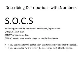
Describing Distributions With Numbers. Section 1.3 (mean, median, range, quartiles, IQR) Target Goal: I can analyze data using shape, center and spread. Hw: pg 70: 79, 80, 81, 84, 87, 89. Measuring Center. Mean ( : x bar ) : The most common measure of center. Median (M).

E N D
Describing Distributions With Numbers Section 1.3 (mean, median, range, quartiles, IQR) Target Goal: I can analyze data using shape, center and spread. Hw: pg 70: 79, 80, 81, 84, 87, 89
Measuring Center Mean ( : x bar): The most common measure of center.
Median (M) The midpoint of a distribution, the # such that half the observations are smaller and the other half are larger.
Resistant Measure (of center) Resists influence of extreme observations. • Mean (average) is not resistant • Median (midpoint) is resistant • The mean and median would be exactly the same if the distribution is exactly symmetric. • In a skewed distribution, the mean is farther out in the long tail then the median.
Ex: Barry BondsFind the median of home runs hit in first 16 seasons. • n= • M= 16 34
How do outliers affect the median? Are there any outliers? If so remove and find M. • n= 15 • Mnew= 34 vs Mold = 34 Median is resistant
How do outliers affect the mean? 16, 19, 24, 25, 25, 33, 33, 34, 34, 37, 37, 40, 42, 46, 49, 73 Find the mean of the original data. • Enter data into L1 • STAT:CALC:1 –Var Stats: L1 • , Mean = 35.44 Find the mean without outlier. • Remove 73 from L1 • STAT:CALC:1 –Var Stats: L1 • Mean = 32.93 We can find median also with 1-Var Stats. Scroll down the list.
Ex: SSHA Scores The Survey of Study Habits and Attitudes (SSHA) is a psychological test that evaluates college students’ motivation, study habits, and attitudes toward school. A private college gives the SSHA to a sample of 18 of its incoming first-year women students. Their scores are:
154 109 137 115 152 140 154 178 101103 126 126 137 165 165 129 200 148154 109 137 115 152 140 154 178 101103 126 126 137 165 165 129 200 148 Make a stemplot of these data. Enter into L2 and sort, then use: • Stems from 10 -20 • Leaves: ones; so 154 looks like 15/4
Are there any potential outliers?About where is the center of the distribution ? 200 Potential outliers: 10 139 Center: 11 5 Median: mean of the 9th and 10thobserv. 12 669 13 77 14 08 15 244 16 55 17 8 18 19 20 0 n = 18 about 138.5
Shape Describe shape: The overall shape of the distribution is irregular, as often happens when only a few observations are available.
Spread What is the spread of the scores (ignoring any outliers)? 178 – 101 = 77 or from 101 to 178
Centerb. : Find the mean score from the formula for the mean. By hand: Sum of the 18 observations/18 = 2539/18 = Calculator keystrokes: 2nd STAT(list):MATH:MEAN(L2) or STAT:CALC:1-Var Stat (L2) = 141.06 141.06
c. Find the median of these scores. Which is larger: the median or the mean? Median = average of the 9th and 10th scores = 138.5 vs. mean = 141.058 Explain why? The mean is larger than the median because of the outlier at 200 whichpulls the mean toward the long right tail of the distribution.
Describe the following distributions: Both distributions are roughly symmetric. The center for both distributions is 90 goals. Both distributions have different amounts of VARIABILITY.
Measuring Spread/Variability • Range: The difference between the largest and smallest observations. • Quartiles: (uses median) The quartiles mark out the middle half and improve our description of spread.
Quartiles 1. Arrange observations in increasing order and locate M. 2.Thefirst quartile (Q1) • lies one-quarter of the way up list of ordered observations • M of lower half • larger than 25% of ordered observations.
3. Thethird quartile (Q3) lies three-quarters of the way up list of ordered observations • larger than 75% of ordered observations. • M of upper half • The “second quartile” • median (M) • Note: is not larger than 50% of ordered observations • is at 50% mark
Barry Bonds cont. Locate Q1 and Q3: Q1 = 25 Q3 = 41
Interquartile Range(IQR): The distance between the first and third quartiles. IQR = Q3 – Q1 IQR = 41 – 25 = 16
Note: If an observation falls in the IQR it is not unusually high or low. We use IQR to identify suspect outliers.
Outliers • Unusually high or unusually low • Basic “rule of thumb” for identifying is if the observation falls more than 1.5 x IQR above the third quartile or below the first quartile.
Outliers • Find IQR • Q3 + 1.5 x IQR (upper cutoff) • Q1 – 1.5 x IQR (lower cutoff)
Is Barry bonds 73 an outlier? • IQR = 41 – 25 = 16 • 1.5 x IQR = = 24 • Q3 + 24 = 41 + 24 = 65(upper cutoff) • Yes or no? Yes Bonds record setting year of 73 is an outlier.
Ex: McDonald’s Chicken Sandwiches Problem: Determine whether the Premium Crispy Chicken Club Sandwich with 28 grams of fat is an outlier. (2 min) Solution: Here are the 14 amounts of fat in order: 9 9 10 10 12 15 16 16 17 17 17 20 23 28
Which is resistant range or IQR? • Range: • IQR: