Download
1 / 34
340 likes | 362 Views
Welfare Implications of the Transition to High Household Debt Jeffrey R. Campbell and Zvi Hercowitz Presentation at the Conference Household Finances and Housing Wealth Banco de España April 2007. Introduction.

E N D
Welfare Implications of the Transition to High Household Debt Jeffrey R. Campbelland Zvi Hercowitz Presentation at the Conference Household Finances and Housing Wealth Banco de España April 2007
Introduction • Who benefits in the economy from relaxing a borrowing constraint? Borrowers or Savers? • Microeconomic level • Macroeconomic level • Relaxation of borrowing constraints in the US: Aggressive deregulation of the mortgage market in early 1980s • Background: • Homes and vehicles collateralize most household debt: 90% in 2001 (1962: 85%). Typical debt contract: equity requirements • Deregulation in 1982: Greater access to sub-prime mortgages and refinancing. Lowering “equity requirements”
Housing equity 1982: 71% of GDP • Household Debt/GDP: 43% in 1983 56% in 1990 • Model: borrower-saver model in Campbell and Hercowitz (2006) • 10th wealth decile. 72.8% of financial assets in 2001 "saver" • 1st-9th wealth deciles. 73.4% of household debt in 2001 "borrower" M
Rest of the Talk • The model • Quantitative results: Computed transition dynamics • Interpretation of the data through the eyes of the model • Welfare effects • Conclusions
The Borrower-Saver Model Main Features • Borrowing is collateralized – equity requirement • The two household differ in time preference and in labor supply. Only the borrower supplies labor • In equilibrium: saver holds all the assets, borrower owes all the debt. Borrower’s only asset: equity on durable goods • The capital stock is constant
Trade Markets are competitive: Households sell capital services and labor to the firms – make loans to each other Factor prices: Ht , Wt Only security traded: Collateralized debt with a period-by-period adjustable rate Notation:
Equity Requirement • Equity requirement parameters: • 0 < < 1: initial equity share • δ≤ < 1: equity accumulation • Required equity share for a good j periods old:
The equity constraint on a household is: This constraint can be rewritten as:
Optimization and Equilibrium • Equity constraint: binds for at most one type of household at a time • Conjecture: It binds for the borrower from t*≥ 0. This is verified in the solution
Utility Maximization by Savers Budget constraint and first-order conditions:
Utility Maximization by Borrowers Constraints:
Quantitative Results The experiment • Initial pre-reform steady state calibrated to the equity requirements observed through 1982:IV • Lower equity requirements: and π values calibrated to the period from 1995:I onwards • Computation of the transition path to the new steady state
loan to value ratio repayment rate Calibration – Main Features Data: Cars: Average loan-to-value ratios and terms from the data Homes: SCF, and actual change in debt/asset ratio High requirement regime: = 0.16, = 0.0315 Low requirement regime: = 0.11, = 0.0186
Computation procedure • Equilibrium path beginning at the old steady state • Modified version of Fair and Taylor's (1983) procedure • Borrower's equity constraint does not bind until t * ≥ 0 • t * = 30
Interpretation of the Evidence • Evolution of wealth distribution from the SCF. Every 3 years: 1983-2001 • Comovement of household debt and interest rates
Shares of the Wealthiest 10% Households(2) Housing and Vehicles
Household Debt and the Real Interest RateDebt/Assets Ratios and Real 3-year T Bill Rate fed
Welfare Analysis • Equivalent permanent change in both consumption goods • Across steady states: • Saver: 12 % • Borrower: -4.4 % • Including the transition: • Saver: 2.02 % • Borrower: 0.26 % • Wage rate, capital income and interest rate constant: • Saver: 0 % • Borrower: 1.35 % • Wage rate and capital income constant: • Saver: 1.36 % • Borrower: 0.45 %
Concluding Comments • The transition is characterized by a prolonged increase in household debt accompanied by high interest rates. • Since 1983: Positive comovement of household debt and interest rates. • The main result: Savers gain from the financial reform more than borrowers---in spite of the fact that the relaxation of equity requirements applies directly to the latter.
Extension of the Model: Irreversible Investment The constraint binds only for the saver, and only initially. t** = 17, t* = 33