Download
1 / 7
70 likes | 261 Views
LECTURE 31: STABILITY OF CT SYSTEMS. Objectives: Stability and the s -Plane Stability of an RC Circuit Routh -Hurwitz Stability Test Step Response of 1 st -Order Systems

E N D
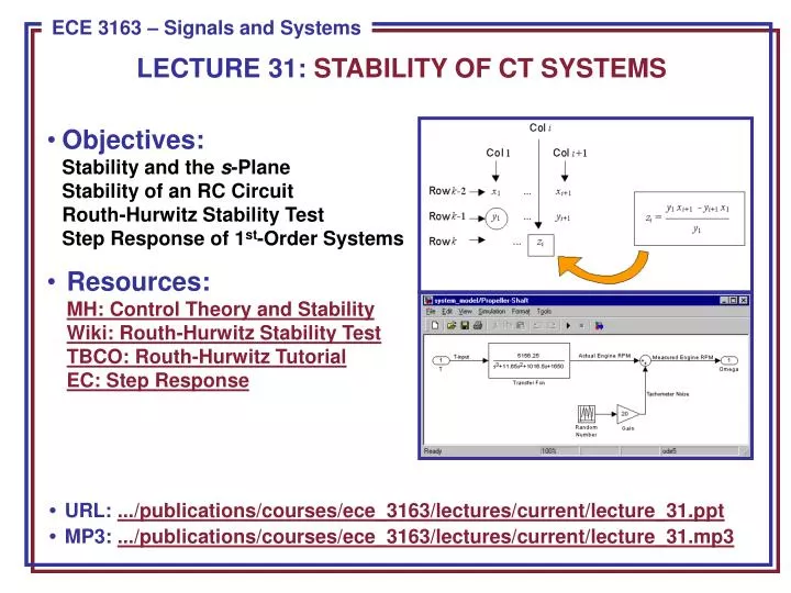
LECTURE 31: STABILITY OF CT SYSTEMS • Objectives:Stability and the s-PlaneStability of an RC CircuitRouth-Hurwitz Stability TestStep Response of 1st-Order Systems • Resources:MH: Control Theory and StabilityWiki: Routh-Hurwitz Stability TestTBCO: Routh-Hurwitz TutorialEC: Step Response • URL: .../publications/courses/ece_3163/lectures/current/lecture_31.ppt • MP3: .../publications/courses/ece_3163/lectures/current/lecture_31.mp3
Stability of CT Systems in the s-Plane • Recall our stability condition for the Laplace transform of the impulse response of a CT linear time-invariant system: • This implies the poles are in the left-half plane.This also implies: • A system is said to be marginally stableif its impulse response is bounded: • In this case, at least one pole of the systemlies on the j-axis. • Recall periodic signals also have poles on the j-axis because they are marginally stable. • Also recall that the left-half plane maps to the inside of the unit circle in the z-plane for discrete-time (sampled) signals. • We can show that circuits built from passive components (RLC) are always stable if there is some resistance in the circuit. LHP
Stability of CT Systems in the s-Plane • Example: Series RLC Circuit • Using the quadratic formula: The RLC circuitis always stable. Why?
The Routh-Hurwitz Stability Test • The procedures for determining stability do not require finding the roots of the denominator polynomial, which can be a daunting task for a high-order system (e.g., 32 poles). • The Routh-Hurwitz stability test is a method of determining stability using simple algebraic operations on the polynomial coefficients. It is best demonstrated through an example. • Consider: • Construct the Routh array: Number of sign changes in 1st column = number of poles in the RHPRLC circuit is always stable
Routh-Hurwitz Examples • Example: • Example:
Analysis of the Step Response For A 1st-Order System • Recall the transfer function for a1st-order differential equation: num = 1; den = [1 –p]; t = 0:0.05:10; y = step(num, den, t); • Define a time constant as the time it takes for the response to reach 1/e (37%) of its value. • The time constant in this case is equal to-1/p. Hence, the real part of the pole, which is the distance of the pole from the j-axis, and is the bandwidth of the pole, is directly related to the time constant.
Summary • Reviewed stability of CT systems in terms of the location of the poles in the s-plane. • Demonstrated that an RLC circuit is unconditionally stable. • Introduced the Routh-Hurwitz technique for determining the stability of a system: does not require finding the roots of a polynomial. • Analyzed the properties of the impulse response of a first-order differential equation. • Next: analyze the properties of a second-order differential equation.