Download
1 / 90
1.01k likes | 1.4k Views
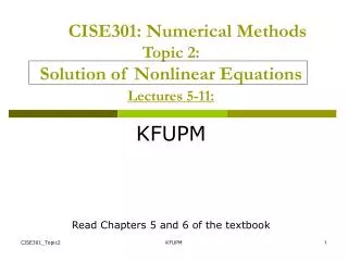
CISE301: Numerical Methods Topic 2: Solution of Nonlinear Equations Lectures 5-11:. KFUPM Read Chapters 5 and 6 of the textbook. Lecture 5 Solution of Nonlinear Equations ( Root Finding Problems ). Definitions Classification of Methods Analytical Solutions Graphical Methods

E N D
CISE301: Numerical MethodsTopic 2: Solution of Nonlinear EquationsLectures 5-11: KFUPM Read Chapters 5 and 6 of the textbook KFUPM
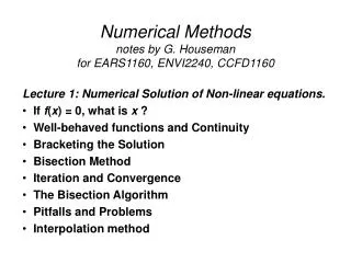
Lecture 5Solution of Nonlinear Equations( Root Finding Problems ) Definitions Classification of Methods Analytical Solutions Graphical Methods Numerical Methods Bracketing Methods Open Methods Convergence Notations Reading Assignment: Sections 5.1 and 5.2 KFUPM
Root Finding Problems Many problems in Science and Engineering are expressed as: These problems are called root finding problems. KFUPM
Roots of Equations A number r that satisfies an equation is called a root of the equation. KFUPM
Zeros of a Function Let f(x) be a real-valued function of a real variable. Any number r for which f(r)=0 is called a zero of the function. Examples: 2 and 3 are zeros of the function f(x) = (x-2)(x-3). KFUPM
Graphical Interpretation of Zeros • The real zeros of a function f(x) are the values of x at which the graph of the function crosses (or touches) the x-axis. f(x) Real zeros of f(x) KFUPM
Simple Zeros KFUPM
Multiple Zeros KFUPM
Multiple Zeros KFUPM
Facts • Any nth order polynomial has exactly n zeros (counting real and complex zeros with their multiplicities). • Any polynomial with an odd order has at least one real zero. • If a function has a zero at x=r with multiplicity m then the function and its first (m-1) derivatives are zero at x=r and the mth derivative at r is not zero. KFUPM
Solution Methods Several ways to solve nonlinear equations are possible: • Analytical Solutions • Possible for special equations only • Graphical Solutions • Useful for providing initial guesses for other methods • Numerical Solutions • Open methods • Bracketing methods KFUPM
Analytical Methods Analytical Solutions are available for special equations only. KFUPM
Graphical Methods • Graphical methods are useful to provide an initial guess to be used by other methods. Root 2 1 1 2 KFUPM
Numerical Methods Many methods are available to solve nonlinear equations: • Bisection Method • Newton’s Method • Secant Method • False position Method • Muller’s Method • Bairstow’s Method • Fixed point iterations • ………. These will be covered in CISE301 KFUPM
Bracketing Methods • In bracketing methods, the method starts with an interval that contains the root and a procedure is used to obtain a smaller interval containing the root. • Examples of bracketing methods: • Bisection method • False position method KFUPM
Open Methods • In the open methods, the method starts with one or more initial guess points. In each iteration, a new guess of the root is obtained. • Open methods are usually more efficient than bracketing methods. • They may not converge to a root. KFUPM
Convergence Notation KFUPM
Convergence Notation KFUPM
Speed of Convergence • We can compare different methods in terms of their convergence rate. • Quadratic convergence is faster than linear convergence. • A method with convergence order q converges faster than a method with convergence order p if q>p. • Methods of convergence order p>1 are said to have super linear convergence. KFUPM
Lectures 6-7Bisection Method The Bisection Algorithm Convergence Analysis of Bisection Method Examples Reading Assignment: Sections 5.1 and 5.2 KFUPM
Introduction • The Bisection method is one of the simplest methods to find a zero of a nonlinear function. • It is also called interval halving method. • To use the Bisection method, one needs an initial interval that is known to contain a zero of the function. • The method systematically reduces the interval. It does this by dividing the interval into two equal parts, performs a simple test and based on the result of the test, half of the interval is thrown away. • The procedure is repeated until the desired interval size is obtained. KFUPM
Intermediate Value Theorem • Let f(x) be defined on the interval [a,b]. • Intermediate value theorem: if a function is continuous and f(a) and f(b) have different signs then the function has at least one zero in the interval [a,b]. f(a) a b f(b) KFUPM
Examples • If f(a) and f(b) have the same sign, the function may have an even number of real zeros or no real zeros in the interval [a, b]. • Bisection method can not be used in these cases. a b The function has four real zeros a b The function has no real zeros KFUPM
Two More Examples • If f(a) and f(b) have different signs, the function has at least one real zero. • Bisection method can be used to find one of the zeros. a b The function has one real zero a b The function has three real zeros KFUPM
Bisection Method • If the function is continuous on [a,b] and f(a) and f(b) have different signs, Bisection method obtains a new interval that is half of the current interval and the sign of the function at the end points of the interval are different. • This allows us to repeat the Bisection procedure to further reduce the size of the interval. KFUPM
Bisection Method Assumptions: Given an interval [a,b] f(x) is continuous on [a,b] f(a) and f(b) have opposite signs. These assumptions ensure the existence of at least one zero in the interval [a,b] and the bisection method can be used to obtain a smaller interval that contains the zero. KFUPM
Bisection Algorithm Assumptions: • f(x) is continuous on [a,b] • f(a) f(b) < 0 Algorithm: Loop 1. Compute the mid point c=(a+b)/2 2. Evaluate f(c) 3. If f(a) f(c) < 0 then new interval [a, c] If f(a) f(c) > 0 then new interval [c, b] End loop f(a) c b a f(b) KFUPM
Bisection Method b0 a0 a1 a2 KFUPM
Example + + - + - - + + - KFUPM
Flow Chart of Bisection Method Start: Given a,b and ε u = f(a) ; v = f(b) c = (a+b) /2 ; w = f(c) no yes is (b-a) /2<ε is u w <0 no Stop yes b=c; v= w a=c; u= w KFUPM
Example Answer: KFUPM
Example Answer: KFUPM
Best Estimate and Error Level Bisection method obtains an interval that is guaranteed to contain a zero of the function. Questions: • What is the best estimate of the zero of f(x)? • What is the error level in the obtained estimate? KFUPM
Best Estimate and Error Level The best estimate of the zero of the function f(x) after the first iteration of the Bisection method is the mid point of the initial interval: KFUPM
Stopping Criteria Two common stopping criteria • Stop after a fixed number of iterations • Stop when the absolute error is less than a specified value How are these criteria related? KFUPM
Stopping Criteria KFUPM
Convergence Analysis KFUPM
Example KFUPM
Example • Use Bisection method to find a root of the equation x = cos (x) with absolute error <0.02 (assume the initial interval [0.5, 0.9]) Question 1: What is f (x) ? Question 2: Are the assumptions satisfied ? Question 3: How many iterations are needed ? Question 4: How to compute the new estimate ? KFUPM
Bisection MethodInitial Interval f(a)=-0.3776 f(b) =0.2784 Error < 0.2 a =0.5 c= 0.7 b= 0.9 KFUPM
Bisection Method -0.3776 -0.06480.2784 Error < 0.1 0.5 0.7 0.9 -0.06480.1033 0.2784 Error < 0.05 0.7 0.8 0.9 KFUPM
Bisection Method -0.06480.0183 0.1033 Error < 0.025 0.7 0.75 0.8 -0.0648 -0.02350.0183 Error < .0125 0.70 0.725 0.75 KFUPM
Summary • Initial interval containing the root: [0.5,0.9] • After 5 iterations: • Interval containing the root: [0.725, 0.75] • Best estimate of the root is 0.7375 • | Error | < 0.0125 KFUPM
A Matlab Program of Bisection Method a=.5; b=.9; u=a-cos(a); v=b-cos(b); for i=1:5 c=(a+b)/2 fc=c-cos(c) if u*fc<0 b=c ; v=fc; else a=c; u=fc; end end c = 0.7000 fc = -0.0648 c = 0.8000 fc = 0.1033 c = 0.7500 fc = 0.0183 c = 0.7250 fc = -0.0235 KFUPM
Example Find the root of: KFUPM
Example KFUPM
Advantages Simple and easy to implement One function evaluation per iteration The size of the interval containing the zero is reduced by 50% after each iteration The number of iterations can be determined a priori No knowledge of the derivative is needed The function does not have to be differentiable Disadvantage Slow to converge Good intermediate approximations may be discarded Bisection Method KFUPM