Download
1 / 64
670 likes | 800 Views
Lecture 3 – Data Summary Measures and Graphical Display of Results. Univariate Data – Analysis of one variable at a time. Why Think About/Explore Data?. Done to accomplish: Checking for data entry errors Describing demographic and study characteristics

E N D
Lecture 3 – Data Summary Measures and Graphical Display of Results Univariate Data – Analysis of one variable at a time
Why Think About/Explore Data? • Done to accomplish: • Checking for data entry errors • Describing demographic and study characteristics • Examining distributions of outcomes • Central tendency • Variability • Checking for outliers • Checking assumptionsfor subsequent analyses • Give a picture of your sample
In order to understand choices of which statistics could be appropriate, it is paramount to ascertain what measurement level the outcome (s) and predictor (s) have. Dependent variable = outcome Independent variable = predictor
Types of Data • Nominal – Qualitative Data Measured in unordered categories • Ordinal – Qualitative Data Measured in ordered categories • Continuous – Quantitative Data Measured on a continuum (summarize with %’s): (summarize with %’s): summarize with Many Summary Measures
Types of Data • Nominal – Qualitative Data Measured in unordered categories • Race • Blood Type • Dead/Alive • Ordinal – Qualitative Data Measured in ordered categories • Cancer Stages • Socio-economic Status (low, med, hi) • Continuous – Quantitative Data Measured on a continuum • Serum Creatinine • Height/Weight/BMI • Gender • On Dialysis/Not on Dialysis • Likert (unlikely, somewhat unlikely, neutral, likely, very likely) • Systolic Blood Pressure • Diastolic Blood Pressure • Others???
Continuous (Numerical) Measures of Location • Mean Arithmetic Average Sum of Values/Number of Values Nice mathematical/statistical properties • Median (a.k.a 50th Percentile) Value where half the sample is above, half the sample is below Better measure for skewed data. Robust to Extreme values • Mode Most Frequently Occurring value in Sample
Continuous (Numerical) NORMAL DISTRIBUTION
Continuous (Numerical) Measures of Variability • Range= (maximum - minimum) • Interquartile range = (Q3 – Q1) always covers half the sample(75th - 25th percentile) • Variance= average of the squares of the deviations of the observations from their mean • Standard deviation=
Continuous (Numerical) NORMAL DISTRIBUTION http://www.stattucino.com/berrie/dsl/index.html
Describing Data using Numerical Summaries • Descriptive statistics: Explore data in order to describe their main features Get an initial picture of data sample
BMI Mean: 32.2 Std: 5.4 Median: 31.8
Mean: 136.3 Std: 17.1 Median: 135
Mean: 189.77 Std: 148.9 Median: 154.11
symmetric skewed to the right skewed to the left Shape of a distribution Mean less than Median (negatively skewed) Mean greater than Median (positively skewed)
Mean: 136.3 Std: 17.1 Median: 135 Skewness: 0.38
Mean: 189.77 Std: 148.9 Median: 154.11 Skewness: 5.63
NORMAL DISTRIBUTION Normal Distribution – Has Excellent Statistical Properties Many Statistical techniques require normal distributions If data does not have Normal Distribution, need to consider alternative techniques appropriate for data
Box (and Whisker) Plots • A graph of the 5 number summary with suspected outliers plotted individually • 5 number summary: • Min, Q1, Median, Q3, Max • A line somewhere inside the box marks the Median • IQR = Q3 – Q1 • Cases more than 1.5*IQR are plotted individually (possible outliers) • Lines from the box extend to the smallest and largest values that are not more than 1.5*IQR
Outlier 1.5 x IQR 75th Percentile median 25th Percentile mean
Skewed to the left Skewed to the right Symmetric + + +
Normal Probability Plot • Plot that can help assess normality. • Idea: plot the observed levels of the variable against the expected levels corresponding to a Normal distribution. • If data lie in a reasonably straight diagonal line, then assumption of Normality is reasonable.
Normal Probability Plots Triglycerides BMI
Error Bar Plots Circle denotes the mean and the bars denote the standard deviation (in this case).
Part II – Measures of Association (plus a little more)
Measures of Association • Continuous Variables • Correlation • Agreement (reliability) • Categorical Variables • Two-way layout (2×2 tables) • “Risk” measures • Agreement • Others
Two Continuous Variables Correlation • General sense: the relationship between two variables (quantitative or qualitative) • Narrow (statistical) sense: measure of interdependence between two continuous random variables • The degree to which increases or decreases in Y occur with increases or decreases in X • Values range between -1 (perfect discordance) and 1 (perfect concordance) • A value of 0 indicates no association
Pearson Correlation Purpose - measures linear association between two continuous variables X and Y Data
Pearson Correlation The Pearson (product-moment) correlation coefficient can be calculated for 2 continuous variables in a sample (regardless of distribution) using the formula:
Correlation Figures Y A B C • • • • • • • • • • • • • • • • • • • • • • • • • • • • • • • ρ = 1 • • • • • ρ = -1 • • • • ρ = 0 X No relationship Perfect positive relationship Perfect negative relationship E D • • • • • • • • • • • • • • • • • • • • • • • • • • ρ = -0.8 • ρ = 0.5 Strong negative relationship Moderate positive relationship
Correlation Inference • Easy “large sample” test for H0: ρ=0 For n ≥ 25, compute which has N(0, ) distribution under H0 • This test assumes X,Y~ NBiv(μX, μY, σX2, σX2, ρ) • Many times a tenuous assumption! • Beware positive skewness & outliers • Beware data not truly continuous
Timeout: ASSUMPTIONS • As with any mathematical or physical model, model assumptions are critical to making the correct inference • Dealing with assumptions has lead to development of: • Nonparametric statistics: techniques that reduce or eliminate dependence on the underlying distribution of the data • Robust statistics: techniques that are affected little by departures from assumptions
Correlation (resumed) • A nonparametric version of the correlation coefficient: Spearman’s Rank Correlation • Like ρ, rs : • ranges from -1 to 1 • 0 no correlation, 1 perfect agreement • only requires ordinal data
Correlation Example: SBP and DBP • All Data: ρ = 0.42; rs = 0.71 • Outlier deleted: ρ = 0.75; rs = 0.82
Correlation Coefficient Questions – • Can we calculate a correlation coefficient between the incomes of a group of people and what city they live in? No, we cannot, since city is a categorical variable. Correlation requires that both variables be quantitative.
Correlation Coefficient Questions – • Does it change the correlation between height and weight if we measure height in inches rather than centimeters and weight in pounds rather than kilograms? No. Because ρ (and r) uses the standardized values of the observations, ρ does not change when we change the units of measurements of x , y, or both. The correlation ρ itself has no unit of measure; it is just a number.
Correlation Coefficient Question – • Does ρ = 0 mean there is no relationship between X and Y ? y • • • • • • • • • • • • • x Correlation only measures the strength of the linear relationship between two variables. Correlation does not describe nonlinear relationships between two variables, no matter how strong they are.
Correlation and Regression Y Y • • • • • • • • • • • • • • • • • • • • • • • • • • ρ = 0.5 ρ = -0.8 • X X Moderate positive relationship Strong negative relationship Y = α+βX
Correlation and Regression SBP and DBP example (continued) σSBP= 4.9 (mmHg) σDBP= 3.3 (mmHg) ρ = 0.75 SBP = 40.1 + 1.12×DBP DBP = 16.3 + 0.51×SBP
Correlation and Covariance • Suppose two random variables, X and Y: E(X) = μX, V(X) = σX2; E(Y) = μY, V(Y) = σY2; and Corr(X,Y) = ρ • Define Cov(X,Y) = E[(X-μX)(Y-μY)] Note: Cov(X,X) = E[(X-μX)(X-μx)] = E(X-μX)2 = σX2 • Population correlation (ρ) is defined as: • Thus Cov(X,Y) = ρσXσY
Correlation and Covariance What’s the big deal about covariance? Use it to find the variance of functions of random variables, e.g.: In general:
Correlation as Agreement Suppose two nurses are measuring SBP in the same patients and each nurse measures SBP 3 times in each patient.