Download
1 / 34
490 likes | 1.4k Views
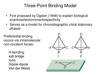
Three Equation Model IS-PC-MR. Monetary Macroeconomics. Motivation for the Model. Over the last decade, many central banks have adopted the policy goal of inflation targeting in the conduct of monetary policy.

E N D
Three Equation ModelIS-PC-MR Monetary Macroeconomics
Motivation for the Model • Over the last decade, many central banks have adopted the policygoal of inflation targeting in the conduct of monetary policy. • Monetary policy is implemented through the use of a nominal interest rate as its policyinstrument. • Traditional macro models make monetary policy actions appear exogenous rather than reflecting the fact that most policy actions represent endogenous reaction to the economy.
Motivation • The model we will study assumes the monetary policy authority (the central bank) acts systematically to minimize fluctuations of output around the full employment level (natural rate) and inflation around its inflation target. • Follows a Taylor Rule.
Key Assumptions of the Model • (1) The inflation process is persistent – slow to change. In line with a wealth of empirical evidence.* • (2) In terms of adjustment lags, assume that it takes one year for monetary policy to affect output and a year for a change in output to affect inflation – 2 years to have an impact on inflation. ------------------------------- * Fed Governors Mishkin and Kroszner have given speeches recently citing studies that showing the inflationary process to be less persistent.
Adjustment Lags • “The empirical evidence is that on average it takes up to about one year in this and other industrial economies for the response to a monetary policy change to have its peak effect on demand and production, and that it takes up to a further year for these activity changes to have their fullest impact on the inflation rate.” ----------------------------------- • Bank of England (1999) The Transmission of Monetary Policy p.9 http://www.bankofengland.co.uk/montrans.pdf
Key Assumptions of the Model • (3) The central bank sets the nominal interest rate (i). But with assumption (1), the expected rate of inflation is given in the short-run, so the central bank can set the real rate (r) in the short-run. (think about why?) Assumption 1: Real Interest rate: From Assumption 1:
The IS - Curve y = C + I + G + (EX – IM) • C = Consumption • I = Investment • G = Government • EX = Exports • IM = Imports • EX – IM = Net Exports • y = real GDP
How does a change in the real interest rate (r) affect spending ? • Asr↑ => C ↓ (Think about why!) => y ↓ • Asr↑ => I ↓ => y ↓ • Asr↑ => EX↓ and IM ↑ => y ↓
The IS–Curve shows an inverse relationship between r and y r IS y
So the Central Bank can adjust r to determine y r r1 r2 r3 IS y1 y2 y3 y If they know the IS-curve relation
So the Central Bank can adjust r to determine y • If it can control the real interest rate, and ( big AND!) 2) If it knows the relationship between r and y • This is to say, it knows the position and the shape of the IS-Curve. Remember, the Fed controls the nominal FFR (iFFR)
Shifts in the IS Curve • We will refer to shifts in the IS curve as “demand shocks” • For example: • Change in I • Change in G • Change in Consumer Confidence => change in C
Shifts in the IS Curve r C↑ I↑ G↑ C ↓ I ↓ G ↓ IS0 IS1 IS2 y
There is a real interest rate (rs) consistent with full employment (ye) r rs A’ IS ye y We will refer to rs as the stabilizing real interest rate. Or the neutral real interest rate (rn in Taylor equation)
Inflation Process (1) (πe = π-1) or (πe = π-1) (2) π = πe + α(y – ye) or (3) π = π-1 + α(y – ye) • Represents inflation inertia. People look backwards in forming expectations => expectations are slow to change. • and (3) state, for a given πe, inflation rises as y rises above full employment (ye ) and falls as y falls below ye . • Question: If y = ye, what can we say about inflation?
Phillips Curve: π = πI + α(y – ye) or Phillips Curve: π = πe + α(y – ye) π VPC (Vertical Phillips Curve) πe = πI = π-1= 2% y > ye π=2% y < ye y ye
Phillips Curve: π = πe + α(y – ye)Movement along the curve π VPC πe = πI= π-1 = 2% π=3% π=2% π=1% y y2 ye y1 When y rises above ye => the output gap ↑ => π↑ When y falls below ye => the output gap ↓ => π↓
Inflation π VPC PC(πe=3) PC(πe=2) 3 πT=2 ye y Shifts in the Phillips Curve: π = πe + α(y – ye)
Figure 1 – Full Employment Equilibrium The economy is at a constant inflation equilibrium output level with y = ye. Inflation is constant at the target rate π =πT = 2%. The stabilizing interest rate is rs. Question: According to the Taylor Rule, what is the nominal FFR (iffr)? VPC
Supply Shock Figure 2 • Suppose an inflation shock (supply shock) takes the economy from A to B. At B there is full employment with high inflation at 4%. • Inflation is above the central bank target level: πT = 2%. • The Fed wishes to reduce inflation to the target level of 2%. B
What does the Phillips Curve show? • The Phillips Curve [PC (πI = 4%)] shows — given last period’s inflation — the inflation and output trade-off faced by the central bank. • The only points on the Phillips Curve with inflation below 4% are to the left of B, i.e. with lower output and hence higher unemployment. • The Fed must create an output gap in order to reduce inflation. • To do this, the Fed must increase the real interest rate.
Figure 3 Figure 3 How does the central bank behave? • The Fed chooses interest rate r'(at point C') causing income to fall to y1. • As y falls, move down along the PC, inflation falls to 3% (why?) • Question: What happens to the PC over time as inflation falls? MR
Monetary Policy Reaction (MR) Function • The Taylor Rule is an example. • A nominal anchor defined in terms of an inflation target provides guidance as to how the real interest rate should be adjusted in response to different shocks hitting the economy. • The objective is stable inflation while minimizing output fluctuations.
The Fed raises the real interest rate to slow down the economy. Inflation falls to 3% • As π falls, people adjust their expectations downward and the PC shifts down to a level consistent with 3% expected inflation. • With lower inflation, the Fed can now adjust the interest rate downward as inflation falls. • The economy moves down the IS curve from C' to D' to A' and along the MR curve from C to D to A. • Eventually the target rate of inflation of 2% is achieved and the economy is at full employment. Figure 4 y1
So what happened here? • The MR line shows the level of output the central bank will choose, given the Phillips curve constraint that it faces. • To implement its output choice, the central bank sets the appropriate interest rate as shown in the IS diagram. • As inflation gradually falls, the Phillips curve shifts down and the central bank chooses an output level closer to the equilibrium. • This traces out the path down the MR along which the economy moves back to equilibrium (i.e. along the MR curve from C to D to A in the Phillips diagram; along the IS curve from C′ to D′ to A′ in the IS diagram).
The Monetary Policy Rule and Central Bank Preference • The more inflation-averse • central bank has a relatively “flat” MR curve. • Starting at point B, such a central bank is prepared to sacrifice a large reduction in output to y1 in order to deliver a given reduction in inflation. • The less inflation-averse central bank has a “steeper” MR curve. This bank is less willing to sacrifice a large fall in output (y2)to deliver a given reduction in inflation. Figure 5 y1 y2
The Monetary Policy Rule and Central Bank Preference Figure 6 • Inflation Shock • Assume there is an inflation shock to the economy that takes inflation to 7%, i.e. to point B and the central bank is faced with the Phillips curve: • PC (πI = 7). • The more inflation-averse • central bank chooses point D on the PC curve, raises the real interest rate to r1 and guides the economy down the MR curve from D to D' to A. y1 y2
The Monetary Policy Rule and Central Bank Preference Figure 6 Inflation Shock The less inflation-averse central bank chooses point F on the PC curve, raises the real interest rate to r2 and guides the economy down the MR curve from F to F' to A. y1 y2
Aggregate Demand Shock • The previous slides show how an inflation shock is handled. • Let’s now look at aggregate demand shocks. The IS curve shifts. • It is assumed that the economy starts off with output at full employment equilibrium and inflation at the target rate of 2%. • Let’s look at a positive aggregate demand shock such as improved consumer expectations: the IS moves to the right to IS′ - a permanent shift. (Fig.7).
Figure 7 Permanent Demand Shock • Output rises above ye (movement from A’ to B’)and inflation will rise above target — in this case to 4%. • As inflationary expectations adjust a new Phillips curve is defined (PC (πI = 4)) along which the central bank must choose its preferred point for the next period: point C. • By going vertically up to point C′ in the IS diagram, the central bank can work out that the appropriate interest rate to set is r′. • The adjustment path down the MR-curve to point Z is exactly as described in the case of the inflation shock.
Permanent Aggregate Demand Shock • This example highlights the role of the stabilizing real interest rate, rS. • Following the shift in the IS curve, there is a new stabilizing interest rate, r's and in order to reduce inflation, the interest rate must be raised above the new r's, for example to r′.
Aggregate Demand Shock • If the demand shock is only temporary, the IS curve shifts to IS′ for only one period before returning to its initial position. • In this case, there is no change to the stabilizing interest rate and the central bank simply raises the real interest relative to the original rS. • This example illustrates the importance for the central bank in being able to forecast the persistence of such shocks.
To Summarize • The rise in output builds a rise in inflation above target into the economy. • Because of inflation inertia, this can only be eliminated by pushing output below and (unemployment above) the equilibrium. • The graphical presentation emphasizes that the central bank raises the interest rate in response to the aggregate demand shock because it can work out the consequences for inflation. The central bank is forward-looking and takes all available information into account. • Its ability to control the economy is limited by the presence of inflation inertia and by the time lag for a change in the interest rate to take effect.
To Summarize • An aggregate demand shock can be fully offset by the central bank even if there is inflation inertia if the central bank’s interest rate decision has an immediate effect on output. • The economy then remains at A in the Phillips diagram in which points A and Z coincide and goes directly from A′ to Z′ in the IS-diagram. This highlights the crucial role of lags and hence of forecasting for the central bank. • The more timely and accurate are forecasts of shifts in aggregate demand, the greater is the chance that the central bank can offset such shocks and prevent the impact of inflation from being built into the economy.


![Structural Equation Model[l]ing (SEM)](https://cdn2.slideserve.com/5132235/slide1-dt.jpg)