Download
1 / 35
350 likes | 629 Views
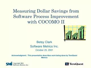
Measuring Dollar Savings from Software Process Improvement with COCOMO II. Betsy Clark Software Metrics Inc. October 25, 2001 Acknowledgment: This presentation describes work being done by TeraQuest Metrics. Outline. Background Measuring the Impact of Software Process Improvement (SPI)

E N D
Measuring Dollar Savings from Software Process Improvement with COCOMO II Betsy Clark Software Metrics Inc. October 25, 2001 Acknowledgment: This presentation describes work being done by TeraQuest Metrics
Outline • Background • Measuring the Impact of Software Process Improvement (SPI) • Some Initial Results
Customer Background • Large financial institution • Actively involved in software process improvement (SPI) • Software-CMM • System Test • Began summer of 2000 at CMM Level 1 • Incrementally adding Key Process Areas • Two pilot organizations • Planning Level 2 assessment end of this year
Background (continued) • Strong emphasis on measuring impact of SPI, especially hard dollar savings • CIO: “If process improvement saves us money, I should be able to go down the street to my competitor’s bank and get a loan to fund our process improvement initiative.”
Outline • Background • Measuring the Impact of Software Process Improvement (SPI) • Some Initial Results • Conclusions
“Maturity levels are meaningless if they cannot be explained in terms of business objectives” John D. VuBoeingLevel 5 Organization
Business Objectives • Reduce the cost of software activities • Reduce delivery time • Improve product quality • Increase customer satisfaction • customers are internal to the bank (e.g., wholesale and retail mortgage, investment division)
Measurement Objectives • Measure impact of SPI in terms of these business objectives • Impacts of SPI will be measured by comparing a set of baseline projects to pilot projects
Measuring Hard Savings • CFO’s initial understanding - • “If we have savings from SPI, we can reduce IT budget in the future.” • First point of discussion - need to measure work load • Led to concept of unit savings, holding IT organization accountable for those savings • Brought IT manager into the discussion - • “But events occur outside of my control that can affect unit costs. For example, I can lose my top staff.”
Measuring Hard Savings • The IT manager was talking about variability due to factors outside of SPI. • That variability is addressed by parametric cost models. • Approach - measure COCOMO II cost drivers for baseline projects and for SPI projects. Use them to adjust unit costs. • Backout all influences on unit costs except SPI
Measuring Hard Savings (cont) • Savings due to SPI • Difference in adjusted unit costs between baseline and SPI projects
Setting Expectations • SPI is a staged, long term initiative • implemented on pilot projects first, then on a wider scale • Initially, we will estimate savings based on pilot results • few data points, wide variation • As SPI is implemented on a wider scale, we will have more data points, clearer trends • Moving from CMM Level 1 to Level 2 lays the foundation for unit cost savings • a few studies do show cost savings from Level 1 to 2 • major effect is in better estimation and planning • reduction in rework due to stable requirements
Measures 1) estimation accuracy: effort 2) estimation accuracy: schedule 3) productivity 4) unit costs 5) project delivery rate (cycle time) 6) system test effectiveness 7) delivered defect density 8) customer satisfaction 9) requirements volatility
Approach • Attempted to “mine” existing data sources (e.g., time tracking, financial, problem reporting systems) • not successful, sporadic and inconsistently used • Selected a representative set of completed projects from the two pilot organizations • Goal was 10-15 projects per pilot organization • 13 projects from one • 11 from the other • Constructed a survey, met with project managers to collect data • Followed-up with each manager to verify data
Measures 1) estimation accuracy: effort 2) estimation accuracy: schedule 3) productivity 4) unit costs 5) project delivery rate (cycle time) 6) system test effectiveness 7) delivered defect density 8) customer satisfaction 9) requirements volatility
Estimation Accuracy - Effort Calculation: (Actual labor hours - estimated) / estimated Overruns Percent difference between actual and estimated 0 Underruns Planned Labor Hours
Estimation Accuracy - Schedule Calculation: (Actual calendar months - estimated) / estimated Overruns Percent Difference between actual and estimated 0 Underruns Planned duration
Measures of Interest • Median - very stable across organizations • standard deviation • Goals with SPI: • median should approach zero • standard deviation should be smaller
Measures 1) estimation accuracy: effort 2) estimation accuracy: schedule 3) productivity 4) unit costs 5) project delivery rate (cycle time) 6) system test effectiveness 7) delivered defect density 8) customer satisfaction 9) requirements volatility
Productivity and Unit Costs • High variability • Median is stable across divisions
Initial Results • Used COCOMO II parameters to adjust size • Led to a reduction in the standard deviation • Helped explain: • why lower productivity projects had difficulty • why higher productivity projects had an easier time • Projects with very high productivity seemed to do everything right • capable staff, low turnover, managing requirements… • these are good things that should improve with SPI • don’t want to penalize organization for improvement in these other (non-SPI) areas • management controllables vs noncontrollables
Measures • 1) estimation accuracy: effort • 2) estimation accuracy: schedule • 3) productivity • 4) unit costs • 5) project delivery rate (cycle time) • 6) system test effectiveness • 7) delivered defect density • 8) customer satisfaction • 9) requirements volatility
Project Delivery Rate • Calculation: • Function points / calendar months • Goal: Increasing
Project Delivery Rate Function points per calendar months Function Points
Measures 1) estimation accuracy: effort 2) estimation accuracy: schedule 3) productivity 4) unit costs 5) project delivery rate (cycle time) 6) system test effectiveness 7) delivered defect density 8) customer satisfaction 9) requirements volatility
System Test Effectiveness • Calculation: • (Defects Found in System Test / Total Defects) • where • Total Defects = (Defects Found in System Test + Delivered Defects found in first 30 days) • Example: • Defects found in System Test = 45 • Defects found in first 30 days of operations = 5 • Test Effectiveness = 90% • Goal: 100% • Result: Wide variation in effectiveness
Measures 1) estimation accuracy: effort 2) estimation accuracy: schedule 3) productivity 4) unit costs 5) project delivery rate (cycle time) 6) system test effectiveness 7) delivered defect density 8) customer satisfaction 9) requirements volatility
Delivered Defect Density • Calculation: • Defects found in first 30 days of operations / function points • Goal: 0
Delivered Defect Density COTS Custom Defects per function points 0 Function Points
(Very Preliminary) Finding of Interest • In contrast to custom development, defect density for COTS projects appears unrelated to size
Measures 1) estimation accuracy: effort 2) estimation accuracy: schedule 3) productivity 4) unit costs 5) project delivery rate (cycle time) 6) system test effectiveness 7) delivered defect density 8) customer satisfaction 9) requirements volatility
Customer Satisfaction, Rqts Volatility • Data do not exist • Strategy was altered to request the manager’s estimate
Message to Executive Level • Measurement • can be a powerful foundation for understanding and managing IT • is a cultural change and not a scoreboard • will improve as process maturity improves
Response from Executive Level (CIO and direct reports) • Intense interest in the measures and in benchmarking • Basis for excellent discussions about need for visibility into • requirements management • quality • customer satisfaction • Collection of the nine measures has been made part of executive compensation • Moving forward to put supporting processes, tools and training in place