Download

1 / 40
410 likes | 761 Views
THE NATURE OF DARK ENERGY FROM N-BODY COSMOLOGICAL SIMULATIONS Paola Solevi Università Milano - Bicocca A.A. 2003/2004. Overview of the talk What is Dark Energy? About n-body cosmological simulations

E N D
THE NATURE OF DARK ENERGY FROM N-BODY COSMOLOGICAL SIMULATIONS Paola Solevi Università Milano - Bicocca A.A. 2003/2004
Overview of the talk • What is Dark Energy? • About n-body cosmological simulations • How to constrain different DE models by n-body cosmological simulations Halos Profile • Halos Mass function • VPF • ICL
What is Dark energy? The best fit model of WMAP: ~70% dark energy • The cosmological constant is described by energy-momentum tensor: • Problems of LCDM cosmology • Coincidence problem: why just now ? • Fine tuning:
Solution: Dynamical Dark energy • We have a real self-interactive scalar filed with a potential • . • Equation of motion • Energy density • Pressure • Potentials which admit a tracker solution: • RPSUGRA Where is the energy scale parameter.
The evolution of the DE density & of time vs. the scale factor
Collision less n-body cosmological simulations • All our simulations are performed using ART, a PM adaptive code (Klypin & Kratsov) and QART, modification of ART (by Andrea Macciò) for models with DDE. • PM (particle-mesh) calculation: • Assign “charge” to the mesh (particle mass grid density) • Solve the field potential equation ( Poisson’s) on the mesh • Calculate the force field from the mesh-defined potential • Interpolate the force on the grid to find forces on the particles • Integrate the forces to get particle velocities and positions • Update the time counter
Basic ingredients Initial conditions: power spectrum of density perturbations depends on the cosmological parameter & inflationary model n=1 for scale-free HZ spectrum is the transfer function (from CMBfast) P(k) at z=40 for different kind of Dark Energy.
FITTING FORMULAE Growing of perturbation depends on the background evolution Analytic formula for in Friedmann eq. for resolving equations used in simulation: (eq. of Poisson ) (eq. of motion)
Linear features of the model Periodic boundary conditions (homogeneity & isotropy), we need a large box for a good representation of the universe Mass & force resolution increase with decreasing box size Nrow number of particles in one dimension Lbox box size Ngrid number of cells in one dimension n number of refinment levels
RP SUGRA LCDM Density profiles All NFW profiles… …but with different concentrations
The best way for test different central concentration is via Strong Gravitational Lensing Formation of Giants Arcs More Arcs for RP model
LCDM Z=0.3 Z=0.5 Z=1.0 Z=1.5 RP
Mass function evolution No differences predicted because of the same σ8 normalization at But different evolution expected z=0
Void probability function Simulations run at HITACHI MUNCHEN MPI 32 Node,32x256 Pr. Three simulations: LCDM, RP (Λ=103GeV), SU (Λ=103GeV)
VPF is a function of all the correlation terms : - reduced n-point correlation function mean value - mean galaxy number in VR Why do we expect that VPF depend on the cosmological model? Different evolution rate Different halo # PLCDM(R)> PSU(R) > PRP(R)
Z=0 VPF, M > 1x10¹²Mʘh-1 Z=0.9 Just as for halos MF no differences predicted at z=0 But different evolution expected
VPF, M > 1x10¹²Mʘh-1 Z=1.5 VPF, M > 5x10¹²Mʘh-1 Notice the dependences on the mass limit, significant differences but halo number getting low
Intracluster light ICL (intracluster light) is due to a diffuse stellar component gravitationally bound not to individual galaxies but to the cluster potential. First ICL Observations : Zwicky 1951 PASP 63, 61 The fraction of ICL depends on the dynamical state of the cluster and on its mass so studying ICL is important to understand the evolution of galaxy clusters. ICL tracers: Red Giants, SNIa, ICG’s,PNe Direct estimations of ICL surface brightness are difficult because it is less than 1% of the sky brightness and because of the diffuse light from the halo of the cD galaxy. Origin: -Tidal stripping -Infall of large groups
Why PNe as ICL tracers? PN is a short (~104 years) phase in stellar evolution between asymptotic giant branch & WD (HR diagram) Because of a so short life, studying PNe’s properties is just like investigating mean local features. The diffuse envelope of a PN re-emits part of UV light from the central star in the bright optical O[III] (λ = 5007 Å) line. Luminosity Surface T
Hot central star T~5x10⁴K Shell of gas from the envelope of central star UV (Arnaboldi et al 2003) O[III] emission
If metallicity is large emission on many lines, scarce efficiency Average efficiency 15% RELATIONSHIP O[III] intensity metallicity age of formation mass Pop I, disk population poor emitters Pop II, bulge population strong emitters
Studying PNe, very low intensity stellar objects are found Cluster materials outside galaxies can be inspected Current studies concentrate on Virgo Main danger in studying PNe: background emitters at λ = 5007 Å contributing ~25% of fake objects (interlopers) Results: - ICPNe not centrally concentrated - 10% < ICL < 40%
Numerical simulations aiming to reproduce the observed PN distribution 1 – Napolitano, Pannella, Arnaboldi, Gehrardt,Aguerri, Freeman, Capaccioli,Ghigna, Governato, Quinn, Stadel 2003 ApJ 594, 172 PKDGRAV n-body cosmological simulation, Model: ΛCDM,Ωm=0.3,σ8=1, h=0.7 Cluster of 3x10¹⁴Mʘ (cluster magnified, still n-body) NO HYDRO
How to use DM to reproduce star formation? Particle in overdensity hits becomes a star - points with at z = 3, 2, 1, 0.5, 0.25, 0 Now for ICL must trace unbound stars - trace points down to z = 0, reject those in subhalos & cD What did they do? - Phase space distribution analysis in 30’x30’ areas at 0.2, 0.4, 0.5, 0.6 Mpc from cluster center - 2-p angular correlation function - Velocity distribution along l.o.s Consistency with observational data
2 – Murante, Arnaboldi, Gehrardt, Borgani, Cheng, Diaferio, Dolag, Moscardini, Tormen, Tornatore, Tozzi ApJL 2004, 607, L83 GADGET (treeSPH) used for LSCS, includes: radiative cooling, SNa feedback, star formation Model: ΛCDM,Ωm=0.3,Ωb=0.019h-2, σ8=0.8, h=0.7 117 clusterswith M > 1014Mʘh-1 HYDRO +
Bound and free stars have been selected by SKID, fraction depends on , optimal ~ 20 h-1kpc Problems with spatial resolution: numerical overmerging causes apparently unbound stars increasing resolution Fraction of unbound stars > 10% (Diemand et al 2003)
3 – Willman, Governato, Wadsley, Quinn astro-ph/0405094 and MNRAS 2004 (in press) GASOLINE (treeSPH) includes: radiative+Compton cooling, SNa feedback, star formation, UV background (Haardt&Madau 1996) Cosmological simulation (n-body) 1 cluster magnified Model: ΛCDM,Ωm=0.3,Ωb not given, σ8=1, h=0.7 HYDRO +
Coma-like galaxy cluster M ~ 1.2x10¹⁵Mʘh-1 (Willman et al 2004) Two large groups ranging in size from Fornax to Virgo
Bound and free stars were detected by SKID using & 20% of stars found in intracluster medium Problem: stellar baryon fraction ~ 36% in simulation vs. 6-10% from 2MASS & SDSS data (Bell et al 2003). COOLING CRISIS: not enough effects to slow down star formation Claim: distribution of stars still OK TRUE? Neglected effects could be star-density dependent Is the sophisticated star formation machinery really better than searching for overdensity regions?
Various conclusions - Unbound stars fraction depends on dynamical status of cluster Two peaks at z~0.55 and z~0.2 correspond to the infall of large groups Variation of IC stars fraction from 10% at z~1 to 22% at z~0 (Willman 2004)
-More IC stars from large galaxies but more star/unit-mass from small galaxies IC fract.from halos M<M (Willman et al 2004) -85% of stars forms at z < 1.1 Mass M
What did we do so far? ART & it’s generalization QART (modified for DE models) Models: ΛCDM Ωm=0.3, σ8=0.75, h=0.7 RP(Λ=103GeV) Ωm=0.3, σ8=0.75, h=0.7 Clusterwith M =2.92x10¹⁴Mʘh-1
LCDM z = 0
RP3 z = 0
LCDM z = 1
RP3 z = 1
LCDM z = 2
RP3 z = 2
Conclusions: What are we doing? - Star formation in iperdensities (SMOOTH), density contrast to be gauged to reproduce observed star amount - Star formation z’s at Δz ~ 0.1 - Dynamical status of candidate-star particle monitorized Extra aim Searching for cosmological model dependencies due to: -different formation history -concentration of dark matter halos