Download
1 / 29
290 likes | 445 Views
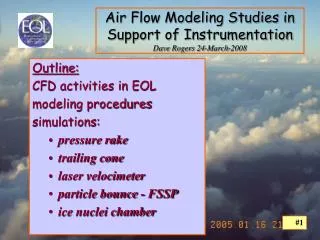
Air Flow Modeling Studies in Support of Instrumentation Dave Rogers 24-March-2008. Outline: CFD activities in EOL modeling procedures simulations: pressure rake trailing cone laser velocimeter particle bounce - FSSP ice nuclei chamber. EOL air flow studies group

E N D
Air Flow Modeling Studies in Support of InstrumentationDave Rogers 24-March-2008 • Outline: • CFD activities in EOL • modeling procedures • simulations: • pressure rake • trailing cone • laser velocimeter • particle bounce - FSSP • ice nuclei chamber
EOL air flow studies group • Cindy Twohy & Dave Rogers • http://www.eol.ucar.edu/raf/Airflow/ • applications: • instrument design • airborne probe placement & alignment • flow & thermodynamics inside of instruments • particle trajectories • improving measurements & their interpretation • identify problems, suggest fixes
software • 1. FLUENT/Gambit • Gambit = geometry & computational mesh • FLUENT = flow solver • http://www.fluent.com/ • 4 licenses • 2. STAR-CD family of programs • Star-CD, pro-am, Star-CCM+, etc. • http://www.cd-adapco.com/ • 10 licenses • Linux & MS-Windows • annual license fees • Tutorial downloads, webinars, training (fee-based) • Both 1 + 2 are user-friendly with graphic user interfaces & menus • Steep learning curve • Frequent use is necessary for proficiency + Plug-in For CAD
What kind of problems can be addressed? • Laminar or turbulent • Compressible • Heat transfer • Multi-phase (evaporating particles, bubbles, melting, freezing, boiling, ..) • Chemical reactions • Steady-state or non-steady (moving grid) • Acoustics • + more … • + user-defined functions
flow simulation steps • build geometry • from basic shapes or import CAD file • create computational mesh • edges, surfaces, volumes • check for quality (size, skewness, ..) • export to flow solver • 3. set boundary conditions (P, T, RH, velocity, ..) • 4. run numerical solver • 5. display results & derived quantities • velocity, pressure, temperature, drag force, .. • particle trajectories, animations
Example 1: BL depth on HIAPER • Scientific need: sample air outside of the flow boundary layer to avoid possible contamination • Advice from Gulfstream: BL = 1% of distance from nose
1:100 Gulfstream laminar flow model
build geometry & mesh • geometry from CAD file import + lots of cleanup • insert into wind tunnel box ~3 m long:7xLong, 3xTall, 8xWide • 540,000 cells
trailing cone • domain ~220,000 cells. • sea level 204 m/s drag force 245 lb.
Example 3:laser velocimeter for HIAPER • (artist’s concept) wing pods
laser velocimeter for HIAPER • domain ~4 x 2 x 2 m3 500,000 cells
cell velocities along horizontal & vertical sections centered on one pod
animation • (change to FLUENT display)
Example 5: ice nuclei chamber Cylinder radii 4 cm & 5 cm. Length 90 cm (airborne); 150 cm (lab). Bottom of outer wall dry or ice-covered. • Description of Chamber • annular space ~1 cm between concentric cylinders • inner walls covered with ice ~ 0.1 mm thick • flow laminar, downward • sample air (1 LPM) slit injection • sheath air (9 LPM) through series of holes
Computational Mesh 5° wedge, 233,000 nodes Full length of model ~1 cm x 90 cm
Parcel Thermodynamic Histories • Earlier 1-D approximation begins with vapor & temperature walls. • FLUENT has dry cold wall & plastic warm wall on first 11 cm then ice coatings begin. These are accurate boundary conditions and indicate slightly different evolution in first 20 cm. • Both studies show response to boundary condition change (dry outer wall) at 62 cm.
Velocity Profiles • FLUENT simulations show flow adjustment occurs through entrance region. At location 42 cm from sample inlet, the FLUENT profile agrees with analytical steady-state solution. • For this case, max velocity ~10 cm/s and contains the sample air lamina.
Particle Trajectories • Outlet cone - no wall loss for dia < 10 µm • Total residence times ~ 11 sec
Recirculation of sheath air Recirculation & Reverse Flow Cold wall • Stagnation region • (small velocities)