Multivariate Toolbox for Linear Model Analysis: Utilizing SVD and MLM for Data Normalization

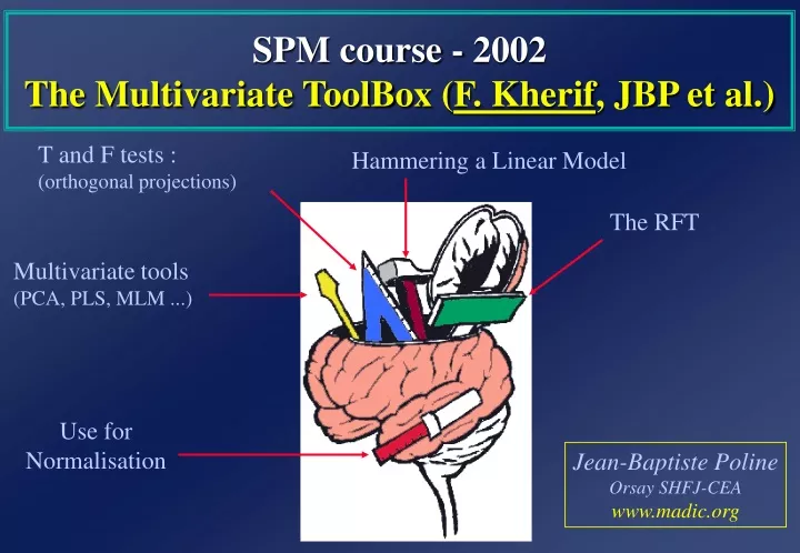
1. SPM course - 2002The Multivariate ToolBox (F. Kherif, JBP et al.) T and F tests : (orthogonal projections) Hammering a Linear Model The RFT Multivariate tools (PCA, PLS, MLM ...) Use for Normalisation Jean-Baptiste Poline Orsay SHFJ-CEA www.madic.org

2. From Ferath Kherif MADIC-UNAF-CEA JB Poline MAD/SHFJ/CEA

3. SVD : the basic concept A time-series of 1D images 128 scans of 40 “voxels” Expression of 1st 3 “eigenimages” Eigenvalues and spatial “modes” The time-series ‘reconstituted’ JB Poline MAD/SHFJ/CEA

4. Eigenimages and SVD V1 V2 V3 voxels APPROX. OF Y U1 U2 APPROX. OF Y U3 APPROX. OF Y s1 + s2 + s3 = + ... Y (DATA) time Y = USVT = s1U1V1T + s2U2V2T + ... JB Poline MAD/SHFJ/CEA

5. Y = X + e ^  Linear model : recall ... voxels parameterestimates =  + residuals design matrix data matrix scans Variance(e) = JB Poline MAD/SHFJ/CEA

6. voxels parameterestimates =  + design matrix residuals data matrix scans Y = X + e Variance(e) = ^  SVD of Y (corresponds to PCA...) V1 V2 U1 U2 voxels APPROX. OF Y APPROX. OF Y s2 s1 + + ... = Y scans [U S V] = SVD (Y) JB Poline MAD/SHFJ/CEA

7. voxels parameterestimates =  + design matrix residuals data matrix scans Y = X + e Variance(e) = ^  SVD of  (corresponds to PLS...) V1 V2 U1 U2 APPROX. OF Y parameterestimates APPROX. OF Y s2 s1 + + ... = [U S V] = SVD (X’Y) JB Poline MAD/SHFJ/CEA

8. voxels parameterestimates =  + design matrix residuals data matrix scans Y = X + e Variance(e) = ^  SVD of residuals : a tool for model checking V1 V2 voxels U1 U2 APPROX. OF Y APPROX. OF Y E s2 scans s1 + + ... = / E / std = normalised residuals JB Poline MAD/SHFJ/CEA

9. Normalised residuals : first component JB Poline MAD/SHFJ/CEA

10. Normalised residuals : first component of a language study Temporal pattern difficult to interpret JB Poline MAD/SHFJ/CEA

11. voxels parameterestimates =  + design matrix residuals data matrix scans Y = X + e Variance(e) = ^  SVD of normalised  (MLM ...) V1 V2 parameterestimates U1 U2 APPROX. OF Y APPROX. OF Y (X’ VX)-1/2 X’ + + ... s1 s2 = [U S V] = SVD ((X’ CX)-1/2 X’Y ) JB Poline MAD/SHFJ/CEA

12. MLM : some good points • Takes into account the temporal and spatial structure without withening • Provides a test • sum of q last eigenvalues Si for q = n, n-1, ..., 1 • find a distribution for this sum under the null hypothesis (Worsley et al) • Temporal and spatial responses : • Yt = Y V’ Temporal OBSERVED response • Xt = X(X’X)-1 (X’ CX)1/2 U’STemporal PREDICTED response • Sp = (X’ CX)-1/2 X’Y U S-1 Spatial response JB Poline MAD/SHFJ/CEA

13. MLM first component p < 0.0001 JB Poline MAD/SHFJ/CEA

14. MLM : more general and computations improved ... • From X’Y to XG’YG XG = X - G(G’G)+G’X YG = Y - G(G’G)+G’Y • X and XG used to need to be of full rank : • not any more • G is chosen through an « F-contrast » that defines a space of interest JB Poline MAD/SHFJ/CEA

15. MLM : implementation • Computation through betas • Several subjects • IN : • An SPM analysis directory (the model has been estimated) IN GENERAL, GET A FLEXIBLE MODEL FOR MLM • A CONTRAST defining a space of interest or of no interest … (here G) IN GENERAL, GET A FLEXIBLE CONTRAST FOR MLM • Output directory • names for eigenimages • OUT : eigenimages, MLM.mat (stat, …) observed and predicted temporal responses; Y’Y JB Poline MAD/SHFJ/CEA

16. Re-inforcement in space ... V1 V2 voxels U1 U2 Subjet 1 Subjet 2 APPROX. OF Y APPROX. OF Y Y s2 + + ... = s1 Subjet n JB Poline MAD/SHFJ/CEA

17. ... or time Subjet 1 V1 U1 voxels Subjet 2 Subjet n APPROX. OF Y s1 Y = V2 U2 + ... + APPROX. OF Y s2 JB Poline MAD/SHFJ/CEA

18. SVD : implementation • Choose or not to divide by the sd of residual fields (ResMS) • removes components due to large blood vessels • Choose or not to apply a temporal filter (stored in xX) • Choose a projector that can be either « in » X or in a space orthogonal to it • study the residual field by choosing a contrast that define the all space • study the data themselves by choosing a null contrast (we need to generalise spm_conman a little) • to detect non modeled sources of variance that may lead to non valid or non optimal data analyses. • to rank the different source of variance with decreasing importance. • Possibility of several subjects JB Poline MAD/SHFJ/CEA

19. SVD : implementation • Computation through the svd(PY’YP’) = v s v’ • compute Y ’Y once, reuse it for an other projector • Y can be filtered or not; divided by the res or not • to get the spatial signal, reread the data and compute Yvs-1 • TAKES A LONG TIME … • possibility of several subjects (in that case, sums the individual Y’Y) • (near) future implementation : use the betas when P projects in the space of X JB Poline MAD/SHFJ/CEA

20. SVD : implementation • IN : • Liste of images (possibly several « subjects ») • Input SPM directory (this is not always theoretically necessary but it is in the current implementation) • A CONTRAST defining a space of interest or of no interest … • in the residual space of that contrast or not ? • Output directory (general, per subject …) • names for eigenimages • OUT : eigenimages, SVD.mat, observed temporal responses; Y’Y; JB Poline MAD/SHFJ/CEA

21. Multivariate Toolbox : An application for model specification in neuroimaging(F. Kherif et al., NeuroImage 2002 ) JB Poline MAD/SHFJ/CEA

22. From Ferath Kherif MADIC-UNAF-CEA JB Poline MAD/SHFJ/CEA

23. JB Poline MAD/SHFJ/CEA

24. Y JB Poline MAD/SHFJ/CEA

25. JB Poline MAD/SHFJ/CEA

26. From Ferath Kherif MAD-UNAF-CEA JB Poline MAD/SHFJ/CEA

27. Subject 1 Subject 2 + Subject 3 - Subject 4 + Subject 5 + Subject 6 + Subject 7 + Subject 8 + Subject 9 + Selected model RESULTS MODEL SELECTION JB Poline MAD/SHFJ/CEA

28. Tr(WiWj) RVij = Sqrt[Tr(Wi2) Tr(Wj2)] D = 1- Rvij , 1 < i,j < k W1=Z1 Z1’ W2= Z2 Z2’ … Wk= Z2 Z2’ Z1=M-1/2 X’Y1 Z2=M-1/2 X’Y2 … Zk=M-1/2 X’Yk Similarity measure Distance matrix Subjects classification (multi-dimensionnal scaling) Group Homogeneity Analysis JB Poline MAD/SHFJ/CEA