Lecture 9 – Radio Astronomy Fundamentals

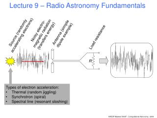
1. Lecture 9 – Radio Astronomy Fundamentals Noisy electro- magnetic radiation (transfers energy) Antenna (simple dipole example) Source (randomly accelerating electrons) Load resistance R • Types of electron acceleration: • Thermal (random jiggling) • Synchrotron (spiral) • Spectral line (resonant sloshing)

2. Noise power spectrum • Analyse the signal into Fourier components. jth component is: • The Fourier coefficient Vj is in general complex-valued. Power in this component is: • Closely related to the ‘power spectrum’ we’ve already encountered in Fourier theory. Vj(t) = Vj exp(-iωjt) = Vj (cos[ωjt] + i sin[ωjt]) Pj = Vj*(t)Vj(t)/R = Vj *Vj/R (cos2[ωjt] + sin2[ωjt]) = Vj *Vj/R

3. Averaging the power spectrum t = 1 t = 16 t = 4 t = 64

4. Total noise power output by the antenna. • “Noise is noise”: signal from an astrophysical source is indistinguishable from contamination from • Background thermal radio noise. • Ditto from intervening atmosphere. • Noise generated in the receiver system. • Each of these makes a contribution to the total. Thus the total noise power is Ptotal = Psource + Pbackground + Patmosphere + Psystem

5. On-and-off source comparison • The simplest way to determine the source contribution is to make 1 measurement pointing at the source, then a second pointing away from (but close to) the source, then subtract the two. • Scanning over the source is also popular. • Uncertainty in total power measurements is: • Note the Poisson-like character: σP is proportional to P. • A low-pass filter with a time constant t is another way of ‘averaging’.

6. Antenna detection efficiency • The source radiates at S W m-2 Hz-1. • The antenna has an effective area Ae in the direction of the source. (Eg for a dish antenna pointed to the source, this is close to the actual area of the dish.) • Thus the power per unit frequency interval picked up by the antenna is: • However, antennas are only sensitive to one polarisation... w = AeS watts per herz.

7. Decomposition into polarised components The total power in the signal is the sum of the power in each polarization. An antenna can only pick up 1 polarization though.

8. Dependence on source polarisation • If the source is unpolarized, the antenna will only pick up ½ the power, regardless of orientation. • If the source is 100% polarized, the antenna will pick up between 0 and 100% of the power, depending on orientation (and type of detector – eg is detector sensitive to linear polarization, or circular). • Obviously all values in between will be encountered. Thus measurement of source polarization is important.

9. Directionality of antennas. A radio telescope often (not always) incorporates a mirror. These are supposed to be smooth mirrors? GMRT An optically ‘smooth’ surface Parkes Ok as long as the roughness is << λ.

10. Directionality of antennas. Radio telescopes with a mirror can be analysed like any other reflecting telescope... Point Spread Function Focal plane Reflector

11. A more usual treatment: It is often conceptually easier to imagine that the antenna is emitting radiation to the sky rather than absorbing it. Side lobe Beam width Side lobe Beam width ~λ/D, same as for any other reflector. Eg Parkes 64m dish at 21 cm, beam width ~ 15’.

12. Going into a little more detail... • Essential quantities: • The distribution of brightness B(θ,φ) over the celestial sphere. (See next slide for definition of θ,φ.) The units of this are W m-2 Hz-1 sr-1 (watts per square metre per herz per steradian). • The effective area Ae of the antenna, in m2. (This is something which must be measured as part of the antenna calibration.) • The relative efficiency f(θ,φ) of the antenna, which is normalized such that it has a maximum of 1. (This shape must also be calibrated.) • The received power spectrum w (units: W Hz-1).

13. Going into a little more detail... Pointing direction of the antenna – NOT the zenith. Kraus uses P where I have f. J D Kraus, “Radio Astronomy” 2nd ed., Fig 3-2.

14. Going into a little more detail... • The general relation between these quantities is: Remember that the ½ only applies where B is unpolarized. • Further useful relations: • It can be shown that ΩA = λ2/Ae.

15. Going into a little more detail... • Let’s consider two limiting cases: • B(θ,φ) = B (ie, uniform over the sky); • B(θ,φ) = Sδ(θ-0,φ-0) (ie, a point source of flux=S, located at beam centre). B(θ,φ)=Sδ B f f w = ½ AeS w = ½ λ2B ...the ½ still applies only for unpolarized B.

16. Conversion of everything to temperatures. • Suppose our antenna is inside a cavity with the walls at temperature T (in kelvin). • It can be shown that the power per unit frequency picked up by the antenna is • Because of this linear relation between a white noise power spectrum and temperature, it is customary in radio astronomy to convert all power spectral densities to ‘temperatures’. Hence: w = kT watts per herz.

17. System temperature • Tsource only says something about the real temperature of the source if • The source area is >>ΩA, and • The physical process producing the radio waves really is thermal. • Tatmosphere is a few kelvin at about 1 GHz. • Tbackground may be as much as 300 K if the antenna is seeing anything of the surroundings! Therefore avoid this. • Tsystem again says nothing about the real temperature of the receiver electronics. Rather it is a figure of merit – the lower the better. Ttotal = Tsource + Tbackground + Tatmosphere + Tsystem

18. The more usual way to write the measurement uncertainty: • Thus the minimum detectable flux is • and the minimum detectable brightness: • Note: • Bmin not dependent on Ae. • Factors of 2 only for unpolarized case.

19. A more realistic system: R M Price, “Radiometer Fundamentals”, Meth. Exp. Phys. 12B (1976), Fig 1, section 3.1.4. “Front end” “Back end”

20. Jargon • The ‘antenna’: • the reflecting surface (ie the dish). • The ‘feed’: • usually a horn to focus the RF onto the detector. • The ‘front end’: • electronics near the Rx (shorthand for receiver). • The ‘back end’: • electronics near the data recorder. • The LO: • local oscillator. A 38 GHz feed horn. The corrugations are good for wide bandwidth. • RF: • Radio Frequency. • IF: • Intermediate Frequency.

21. Flux calibration • The bandwidth and gain of the radiometer tend not to be very stable. • There are several methods of calibration. Eg: • Switching between the feed and a ‘load’ at a temperature similar to the antenna temperature. But, this can be < 20 K... • Periodic injection of a few % of noise into the feed. Noise sources can be made much more stable than noise detectors. • Still good to look occasionally at an astronomical source of known, stable flux. Should also be unresolved (compact). • Difficult conditions to meet all together! Compact sources tend to vary with time.