Constant-Working Space Algorithms for Image Procesing
420 likes | 448 Views
Explore constant-working-space algorithms for image processing applications embedded in hardware, developing efficient solutions in a limited storage framework. Discover approaches and applications to image thresholding and intensity image processing. Learn about algorithms and techniques like median-finding and optimal thresholding. Find out how to find the median and optimize image processing tasks using a restricted working space, with practical examples and analysis.

Constant-Working Space Algorithms for Image Procesing
E N D
Presentation Transcript
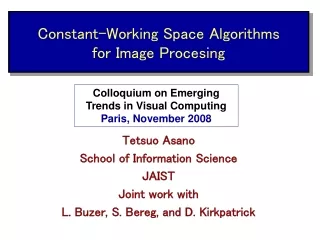
Constant-Working Space Algorithmsfor Image Procesing Colloquium on Emerging Trends in Visual Computing Paris, November 2008 Tetsuo Asano School of Information Science JAIST Joint work with L. Buzer, S. Bereg, and D. Kirkpatrick
What is a constant-working-space algorithm? • Input data are given on a read-only array. • Only constant number of working storage cells are available. • Each working storage cell is of O(log n) bits, and hence the total working storage size is also O(log n). • A class of problems solved in this framework is known as log-space in complexity theory. • Want to develop efficient algorithms in this computational model.
Why constant-working-space? • Working space is limited in applications to software embedded in hardware: e.g.: scanner, digital camera, etc. • In some applications we want to keep input data unchanged data on a read-only array. • Recursion working space ∝ recursion depth algorithmic techniques such as controlled recursion.
What is known? • Median-finding: Given a read-only array of n numbers, find their median using constant number of variables. Munro-Raman, Theoretical Computer Science, 1996. • st-connectivity in graph: Given an undirected graph using a read-only array, determine whether two arbitrarily given vertices belong to the same connected component. Reingold, STOC, 2005. • st-connectivity in image: Given a read-only array of a binary image, determine whether two arbitrarily specified pixels of the same value belong to the same connected component. Malgouyresa-Moreb, Theoretical Computer Science, 2002.
st-connectivity in maze t s Is s connected to t? checked by right-hand rule
st-connectivity in maze removed boundary cells t s t Is s connected to t?
st-connectivity in maze t s t Is s connected to t? cannot be checked by right-hand rule
st-connectivity in a graph s t Is there any path from s to t? A graph is given using a read-only array.
st-connectivity in a graph s t Is there any path from s to t? A graph is given using a read-only array.
st-connectivity in a binary image 0000000011000111000 0011100000111100011 0111111000000111111 0110011110001110000 0111110011100111111 t s Is there any rectilinear path of white pixels (of values 1) interconnecting s to t?
st-connectivity in a binary image 0000000011000111000 0011100000111100011 0111111000000111111 0110011110001110000 0111110011100111111 t s Is there any rectilinear path of white pixels (of values 1) interconnecting s to t?
Median-finding 1 13 5 31 9 3 25 39 35 11 6 20 27 13 17 sorted seq: 3, 5, 6, 9, 11, 13, 17, 20, 25, 27, 31, 35, 39 median Linear-time algorithm based on prune and search, Blum, Floyd, Pratt, Rivest, Tarjan, 1972. How fast can we find the median in the computational model? O(n) time? O(n log n) time? W(n2) time?
Algorithm A3 Partition the array into n1/3 blocks instead of n1/2 blocks. Compute a block median using Algorithm A2. Algorithm A3 finds the median in O(n4/3 log2 n) time using only constant working space. Algorithm Ak Partition the array into n1/k blocks. Compute a block median using Algorithm Ak-1. Algorithm Akfinds the median in O(n(k+1)/k logk-1 n) time using O(k) working space.
Applications to Image Processing Thresholding Intensity Images Given an intensity image G, find an appropriate threshold for G to generate a good-looking binary image. threshold=100 too low threshold=150 intensity image too high each threshold is to be evaluated by the resulting binary image. The input image should be treated as a read-only array.
100 128 150 200 threshold =50 a binary image looking best intensity image
a binary image looking best intensity image threshold 50 100 150 200
Average intensity level of each class discriminant analysis: inter-cluster distance max Ohtsu's Optimal Thresholding Divide a given histogram into two classesS0, S1at a threshold t class S0 class S1 Choose a threshold t so that their difference is maximized by considering balance of their areas.
Criterion in the discriminant analysis (by Ohtsu) inter-cluster distance n(Si) = size of Class i (number of pixels) m(Si) = average intensity level of Class i mT = average intensity level of the whole image Choose a threshold t that minimizes V(t) as an optimal threshold (Note: an optimal threshold can be computed in linear time)
Observation: Let n be the number of pixels in a given image and L be the number of intensity levels. Given such an image, we can find in O(n + L) time using O(L) space in addition to the image array an optimal threshold that maximizes the intercluster distance. If O(L) working space is not available we rely on binary search for an optimal threshold. intercluster distance max all these values can be computed using constant working space.
Observation: Let n be the number of pixels in a given image and L be the number of intensity levels. Given such an image, we can find in O(n log L) time using only constant working space in addition to the image array an optimal threshold that maximizes the intercluster distance. Remark: The binary search works only when intensity levels are given by integers 1..L. What happens if all intensity levels are real numbers? Median intensity level instead of Ohtsu's threshold. O(n1+e) time algorithm using O(1/e) working space.
thresholding Experimental results
Histogram Computation Problem: Let G be a monochrome image containing n pixels, and L be the number of intensity levels. Given such an image, report the frequency of each intensity level. histogram computation Easy solution: If O(L) working storage is available, then it is done in O(n) time. What about the case of constant working space? O(k) working storage => O(nL/k) time using O(k) working space inefficient if L >> n.
Constant working space algorithm for histogram computation Let Q be a priority queue keeping O(k) values together with their frequencies in the decreasing order of their keys. T = positive infinity do{ for each pixel (x, y) in a given image if its the intensity level p(x, y) is less than T then put it into Q report the content of the queue Q T = the smallest key value in Q } while(Q is not empty) This algorithm runs in O(n2/k log k) time using O(k) space.
Connected Components Counting What is a connected component? M: an nxn binary image (matrix) M(x, y) = 0 or 1 Two 1-pixels are connected if there is a rectilinear sequence of 1-pixels between them. A connected component is a maximal set of 1-pixels any two of which are connected.
Theorem: There is a constant working space algorithm for connected components labeling in linear time which put labels onto the input image without using any other working storage. linear-time in-place algorithm for connected components labeling linear-time in-place algorithm for counting connected components What about the case when input image is given as a read-only array?
Key Idea for Counting Basic assumption: Component boundary is directed so that the interior always lies to the left of the boundary External boundary : counter-clockwise order Internal boundary : clockwise order
Key Idea for Counting Basic assumption: Component boundary is directed so that the interior always lies to the left of the boundary External boundary : counter-clockwise order Internal boundary : clockwise order Canonical edge for each boundary: the lowest downward edge
Each boundary (internal/external) has a unique canonical edge, which is the lowest downward edge on the boundary.
Local configuration around a starting edge 0 0 1 1 0 1 External boundary Internal boundary Checking orientation So easy to check the orientation!!
Algorithm for Connected Components Counting counter = 0. Perform Raster Scan whenever we find a candidate downward edge e. Apply Boundary_trace_from(e). if it returns 1 then increment the count Report the count. 0 1 ? 0 Boundary_trace_from(e){ es = e. do{ e = next edge of e on the same boundary. if e is downward and lower than es then return 0. }while(e != es) return 1. }
Theorem: The algorithm Connected-Components-Counting correctly computes the number of connected components in a given nxn binary image in O(n4) time using only constant amount of working storage. worst-case example
How to improve the time complexity bidirectional search whenever we find a candidate edge e, search on the boundary in two opposite directions for any lower edge. Now, it is an easy case.
How to improve the time complexity bidirectional search whenever we find a candidate edge e, search on the boundary in two opposite directions for any lower edge. worst-case example which requires O(n2log n)
Enumeration of all components together with their areas Given a binary image G, enumerate all connected components together with their areas (number of pixels) each exactly once. input output component 1 21 component 2 3 component 3 7 component 4 15 Question: Can we obtain such a list in a read-only model?
Enumeration of all components together with their areas Given a binary image G, enumerate all connected components together with their areas (number of pixels) each exactly once. There is a constant-working-space algorithm for enumerating all components together with their areas for a read-only array for a binary image which runs in O(n2 log n) time.
Pattern Matching Given two binary images G1 and G2, determine whether a pattern in G1 appears in G2. pattern G1 given image G2
1 1 1 0 0 1 1 0 holes, islands, island hole canonical edges, candidates detecting an internal boundary search within the external boundary search within the internal boundary
search within the external boundary search OUTSIDE the external boundary detection of an internal boundary and then search within it search within the external boundary
detection of an internal boundary and then search within it completing the search on the external boundary, and then returning to the previous boundary continue the search: detecting a new boundary
Conclusions and Future Works • Extend the algorithm for geometric problems such as planar subdivisions or graphs. • Establish some non-linear lower bound on the time complexity for constant-working-space algorithms: element uniqueness, sorting, largest gap? • Devise more algorithmic paradigms for constant-working-space algorithms
Thank you! Kenrokuen Garden, Kanazawa, Japan