Transfer Learning Algorithms for Image Classification
Transfer Learning Algorithms for Image Classification. Ariadna Quattoni MIT, CSAIL. Advisors: Michael Collins Trevor Darrell. Motivation. Goal:. We want to be able to build classifiers for thousands of visual categories. We want to exploit rich and complex feature representations.

Transfer Learning Algorithms for Image Classification
E N D
Presentation Transcript
Transfer Learning Algorithms forImage Classification Ariadna Quattoni MIT, CSAIL Advisors: Michael Collins Trevor Darrell
Motivation Goal: • We want to be able to build classifiers for thousands of visual categories. • We want to exploit rich and complex feature representations. Problem: • We might only have a few labeled samples per category. Solution: • Transfer Learning, leverage labeled data from multiple related tasks.
Thesis Contributions We study efficient transfer algorithms for image classification which can exploit supervised training data from a set of related tasks: • Learn an image representation using supervised data from auxiliary tasks automatically derived from unlabeled images + meta-data. • A transfer learning model based on joint regularization and an efficient optimization algorithm for training jointly sparse classifiers in high dimensional feature spaces.
A method for learning image representations fromunlabeled images + meta-data Large dataset of unlabeled images + meta-data Visual Representation Structure Learning [Ando & Zhang, JMLR 2005] Create auxiliary problems • Structure Learning: Task specific parameters Shared Parameters
A method for learning image representations fromunlabeled images + meta-data
Outline • An overview of transfer learning methods. • A joint sparse approximation model for transfer learning. • Asymmetric transfer experiments. • An efficient training algorithm. • Symmetric transfer image annotation experiments.
Transfer Learning: A brief overview • The goal of transfer learning is to use labeled data from related tasks to make learning easier. Two settings: • Asymmetric transfer: Resource: Large amounts of supervised data for a set of related tasks. Goal: Improve performance on a target task for which training data is scarce. • Symmetric transfer: Resource: Small amount of training data for a large number of related tasks. Goal: Improve average performance over all classifiers.
Transfer Learning: A brief overview • Three main approaches: • Learning intermediate latent representations: [Thrun 1996, Baxter 1997, Caruana 1997, Argyriou 2006, Amit 2007] • Learning priors over parameters: [Raina 2006, Lawrence et al. 2004 ] • Learning relevant shared features [Torralba 2004, Obozinsky 2006]
Feature Sharing Framework: • Work with a rich representation: • Complex features, high dimensional space • Some of them will be very discriminative (hopefully) • Most will be irrelevant • Related problems may share relevant features. • If we knew the relevant features we could: • Learn from fewer examples • Build more efficient classifiers • We can train classifiers from related problems together using a regularization penalty designed to promote joint sparsity.
Grocery Store Flower-Shop Church Airport
Grocery Store Flower-Shop Church Airport
Grocery Store Flower-Shop Church Airport
Related Formulations of Joint Sparse Approximation • Obozinski et al. [2006] proposed L1-2 joint penalty and developed a blockwise boosting scheme based on Boosted-Lasso. • Torralba et al. [2004] developed a joint boosting algorithm based on the idea of learning additive models for each class that share weak learners.
Our Contribution A new model and optimization algorithm for training jointly sparse classifiers: • Previous approaches to joint sparse approximation have relied on greedy coordinate descent methods. • We propose a simple an efficient global optimization algorithm with guaranteed convergence rates. • Our algorithm can scale to large problems involving hundreds of problems and thousands of examples and features. • We test our model on real image classification tasks where we observe improvements in both asymmetric and symmetric transfer settings.
Outline • An overview of transfer learning methods. • A joint sparse approximation model for transfer learning. • Asymmetric transfer experiments. • An efficient training algorithm. • Symmetric transfer image annotation experiments.
Notation Collectionof Tasks Joint Sparse Approximation
Single Task Sparse Approximation • Consider learning a single sparse linear classifier of the form: • We want a few features with non-zero coefficients • Recent work suggests to use L1 regularization: L1 penalizes non-sparse solutions Classification error • Donoho [2004] proved (in a regression setting) that the solution with smallest L1 norm is also the sparsest solution.
Joint Sparse Approximation • Setting : Joint Sparse Approximation Penalizes solutions that utilize too many features Average Loss on Collection D
Joint Regularization Penalty • How do we penalize solutions that use too many features? Coefficients for for feature 2 Coefficients for classifier 2 • Would lead to a hard combinatorial problem .
Joint Regularization Penalty • We will use a L1-∞ norm [Tropp 2006] • This norm combines: The L∞norm on each row promotes non-sparsity on each row. Share features An L1 norm on the maximum absolute values of the coefficients across tasks promotes sparsity. Use few features • The combination of the two norms results in a solution where only a few features are used but the features used will contribute in solving many classification problems.
Joint Sparse Approximation • Using the L1-∞normwe can rewrite our objective function as: • For any convex loss this is a convex objective. • For the hinge loss: the optimization problem can be expressed as a linear program.
Joint Sparse Approximation • Linear program formulation (hinge loss): • Max value constraints: and • Slack variables constraints: and
Outline • An overview of transfer learning methods. • A joint sparse approximation model for transfer learning. • Asymmetric transfer experiments. • An efficient training algorithm. • Symmetric transfer image annotation experiments.
Setting: Asymmetric Transfer SuperBowl Sharon Danish Cartoons Academy Awards AustralianOpen Trapped Miners Golden globes • Train a classifier for the 10th held out topic using the relevant features R only. Figure Skating Iraq Grammys • Learn a representation using labeled data from 9 topics. • Learn the matrix W using our transfer algorithm. • Define the set of relevant features to be:
Outline • An overview of transfer learning methods. • A joint sparse approximation model for transfer learning. • Asymmetric transfer experiments. • An efficient training algorithm. • Symmetric transfer image annotation experiments.
Limitations of the LP formulation • The LP formulation can be optimized using standard LP solvers. • The LP formulation is feasible for small problems but becomes intractable for larger data-sets with thousands of examples and dimensions. • We might want a more general optimization algorithm that can handle arbitrary convex losses.
L1-∞ Regularization: Constrained Convex Optimization Formulation A convex function Convex constraints • We will use a Projected SubGradient method. Main advantages: simple, scalable, guaranteed convergence rates. • Projected SubGradient methods have been recently proposed: • L2 regularization, i.e. SVM [Shalev-Shwartz et al. 2007] • L1 regularization [Duchi et al. 2008]
Characterization of the solution Feature I Feature II Feature III Feature VI
Mapping to a simpler problem • We can map the projection problem to the following problem which finds the optimal maximums μ:
Efficient Algorithm for: , in pictures 4 Features, 6 problems, C=14
Complexity • The total cost of the algorithm is dominated by a sort of the entries of A. • The total cost is in the order of:
Outline • An overview of transfer learning methods. • A joint sparse approximation model for transfer learning. • Asymmetric transfer experiments. • An efficient training algorithm. • Symmetric transfer image annotation experiments.
Synthetic Experiments • Generate a jointly sparse parameter matrix W: • For every task we generate pairs: where • We compared three different types of regularization (i.e. projections): • L1−∞ projection • L2 projection • L1 projection
Synthetic Experiments Performance on predicting relevant features Test Error
Dataset: Image Annotation president actress team • 40 top content words • Raw image representation: Vocabulary Tree (Grauman and Darrell 2005, Nister and Stewenius 2006) • 11000 dimensions
Results The differences are statistically significant
Dataset: Indoor Scene Recognition bakery bar Train station • 67 indoor scenes. • Raw image representation: similarities to a set of unlabeled images. • 2000 dimensions.
Summary of Thesis Contributions • A method that learns image representations using unlabeled images + meta-data. • A transfer model based on performing a joint loss minimization over the training sets of related tasks with a shared regularization. • Previous approaches used greedy coordinate descent methods. We propose an efficient global optimization algorithm for learning jointly sparse models. • A tool that makes implementing an L1−∞ penalty as easy and almost as efficient as implementing the standard L1 and L2 penalties. • We presented experiments on real image classification tasks for both an asymmetric and symmetric transfer setting.
Future Work • Online Optimization. • Task Clustering. • Combining feature representations. • Generalization properties of L1−∞ regularized models.