Download
1 / 28
280 likes | 304 Views
Addressing the growing energy demand in microprocessors, this study explores power-performance tradeoffs through dynamic voltage and frequency scaling in MPI programs. It implements an adaptive system for efficient power usage by identifying reducible code regions and adjusting CPU states accordingly. The work examines the impact of automatic p-state transitions on energy efficiency and performance in MPI communication phases, offering insights for future optimization strategies.

E N D
Adaptive, Transparent Frequency and Voltage Scaling of Communication Phases in MPI Programs Min Yeol Lim Computer Science Department Sep. 8, 2006
Growing energy demand • Energy efficiency is a big concern • Increased power density of microprocessors • Cooling cost for heat dissipation • Power and performance tradeoff • Dynamic voltage and frequency scaling (DVFS) • Supported by newer microprocessors • Cubic drop on power consumption • Power frequency × voltage2 • CPU is the major power consumer : 35~50% of total power
Power-performance tradeoff • Cost vs. Benefit • Power performance • Increasing execution time vs. decreasing power usage • CPU scaling is meaningful only if benefit > cost P1 E = P1 * T1 Benefit Power P2 E = P2 * T2 Cost T1 T2 Time
Power-performance tradeoff (cont’) • Cost > Benefit • NPB EP benchmark • CPU-bound application • CPU is on critical path • Benefit > Cost • NPB CG benchmark • Memory-bound application • CPU is NOT on critical path 0.8Ghz 1.2 1.6 1.0 2.0 1.4 1.8
Motivation 1 • Cost/Benefit is code specific • Applications have different code regions • Most MPI communications are not critical on CPU • P-state transition in each code region • High voltage and frequency on CPU intensive region • Low voltage and frequency on MPI communication region
Time and energy performance of MPI calls • MPI_Send • MPI_Alltoall
Motivation 2 • Most MPI calls are too short • Scaling overhead by p-state change per call • Up to 700 microseconds in p-state transition • Make regions with adjacent calls • Small interval of inter MPI calls • P-state transition occurs per region Fraction of intervals Fraction of calls Call length (ms) MPI calls interval (ms)
R1 R2 R3 Reducible regions user MPI library A B C D E F G H I J time
Reducible regions (cont’) • Thresholds in time • close-enough (τ): time distance between adjacent calls • long-enough (λ): region execution time δ < τ δ < τ δ > λ user MPI library A B C D E F G H I J time
How to learn regions • Region-finding algorithms • by-call • Reduce only in MPI code: τ=0, λ=0 • Effective only if single MPI call is long enough • simple • Adaptive 1-bit prediction by looking up its last behavior • 2 flags : begin and end • composite • Save patterns of MPI calls in each region • Memorize the begin/end MPI calls and # of calls
P-state transition errors • False-positive (FP) • P-state is changed in the region top p-state must be used • e.g. regions terminated earlier than expected • False-negative (FN) • Top p-state is used in the reducible region • e.g. regions in first appearance
Optimal transition top p-state reduced p-state top p-state Simple reduced p-state Composite top p-state reduced p-state P-state transition errors (cont’) A B A B A B Program execution users MPI library FN FN
Optimal transition top p-state reduced p-state top p-state Simple reduced p-state Composite top p-state reduced p-state P-state transition errors (cont’) A A A A A A Program execution users MPI library FP FP FP F N FN
Selecting proper p-state • automatic algorithm • Use composite algorithm to find regions • Use hardware performance counters • Evaluation of CPU dependency in reducible regions • A metric of CPU load: micro-operations/microsecond (OPS) • Specify p-state mapping table
Implementation • Use PMPI • MPI profiling interface • Intercept pre and post hooks of any MPI call transparently • MPI call unique identifier • Use the hash value of all program counters in call history • Insert assembly code in C
Results • System environment • 8 or 9 nodes with AMD Athlon-64 system • 7 p-states are supported: 2000~800Mhz • Benchmarks • NPB MPI benchmark suite • C class • 8 applications • ASCI Purple benchmark suite • Aztec • 10 ms in thresholds (τ, λ)
Benchmark analysis • Used composite for region information
Taxonomy • Profile does not have FN or FP
Comparison of p-state transition errors • Breakdown of execution time Simple Composite
τ evaluation • SP benchmark
τ evaluation (cont’) MG CG BT LU
Conclusion • Contributions • Design and implement an adaptive p-state transition system in MPI communication phases • Identify reducible regions on the fly • Determine proper p-state dynamically • Provide transparency to users • Future work • Evaluate the performance with other applications • Experiments on the OPT cluster
State transition diagram • Simple begin == 1 else else OUT IN end == 1 not “close enough” “close enough”
State transition diagram (cont’) • Composite else not “close enough” OUT not “close enough” end of region operation begins reducible region “close enough” IN REC else “close enough” pattern mismatch
Benchmark analysis • Region information from composite with τ = 10 ms