Advanced Grid Methods for Weather Forecasting
Explore the Gridded MOS station analysis for various weather elements using regional operator equations and correction methods. Learn about elevation adjustments, smoothing algorithms, and error checking techniques.

Advanced Grid Methods for Weather Forecasting
E N D
Presentation Transcript
GRIDDED MOS • STARTS WITH POINT (STATION) MOS • Essentially the same MOS that is in text bulletins • Number and type of stations differ for different weather elements
MOS Stations available to analysis METAR Elements • Probability of Precipitation • QPF
MOS Stations available to analysis METAR, Marine Elements • Sky Cover • Wind Gusts
MOS Stations available to analysis METAR, Marine, Mesonet Elements • Wind Direction • Wind Speed • 2-m Temperature • 2-m Dew Point • Relative Humidity
MOS Stations available to analysis METAR, Marine, Mesonet, COOP, RFC Elements • Daytime Maximum Temperature • Nighttime Minimum Temperature
TWO METHODS OF PROVIDING GRIDDED MOS • Develop in such a way that forecasts can be produced directly at gridpoints • Regional Operator Equations (RO) • Generalized Operator Equations (GO) - (One big region) • RO and GO forecasts not as accurate as single station • RO equations applied to a fine scale grid produce discontinuities between regions • Develop for and apply at stations, and grid them • Successive Correction analysis (e.g., Cressman, Barnes) • Relatively simple and fast • Details of application vary with weather element • One or more passes over data, correcting the “current” grid by an amount determined by the difference between the analysis and the forecast
SUCCESSIVE CORRECTION • Start with first guess • Can be a constant (generally doesn’t matter what constant, except for error checking (e.g., a specified constant or the average of all values to be analyzed), or can be, for instance, a similar model field • Current analysis value at a station determined by interpolation (bilinear) • Difference between current analysis and forecast, with possibly an elevation correction, determines correction at nearby gridpoints within a radius of influence R according to one of three algorithms • R varies by pass • Approximately 35 to 40 on first pass and 15 to 20 on last pass
CORRECTION METHODS • 3 Possible types of correction for each gridpoint • 1) Average contribution from all stations • 2 Weight contributions from all stations by distance between station and gridpoint • 3) Same as 2), except divide sum by sum of weights • No. 3 used almost exclusively
SMOOTHING ALGORITHM • Basic method • Average the point to be smoothed with average of the surrounding 4 (or 8) points, weighting the average by a specified factor • Terrain-Following • Smoothing is not done across significant valleys and ridges (> 100 m elevation difference across the valley or ridge • Smoothing across an island or spit of land is not done • Only land points involved in smoothing of land gridpoints • Only water points involved in smoothing of water gridpoints • High and low values for the forecasts can be smoothed or not with either 5- or 9-point smoother, depending on weather element and terrain differences.
ELEVATION ADJUSTMENT • Based on average lapse rate at pairs of stations • Each station has a list of 60 to 100 neighboring stations that are close in horizontal distance but far apart in elevation • Neighboring stations determined by preprocessing the metadata and remain the same for all analyses • When analyzing, many of these neighbors may be missing, so lapse rate may not be calculated if too few neighbors • Lapse rate for each station is the sum of all forecast differences divided by the sum of elevation differences • Pair always > 130 m separation in the vertical • Pair may be up to 337.5 km away
ELEVATION ADJUSTMENT • Strength of elevation adjustment varies by pass • Generally full adjustment on Pass 1, with lesser on following passes • Last pass may have no adjustment • Adjustment can be both up and down, or only one way • Elevation adjustment may not be used for some weather elements (e.g., U and V wind—used only for direction)
ELEVATION ADJUSTMENT • “Unusual” lapse rates are limited • By strength of adjustment • By distance • Temperature change with elevation usually negative, but may be positive along the west coast • “Unusual” defined for each weather element
Unusual Lapse Rates
WATER VERSUS LAND • Gridpoints are designated as either (1) Ocean, (2) Inland Water, or (3) Land • Stations are designated as either (1) Ocean, (2) Inland Water, (3) Land, or (4) Both land and inland water • Each type of station affects a corresponding type of gridpoint • Essentially three analyses in one • Interpolation recognizes difference
ERROR CHECKING • Threshold defined for each weather element for each analysis pass • Difference between the current analysis and the forecast must be < the threshold for the forecast to be used on that pass • But--Before discarding when threshold is not met, two nearest neighbors are checked, both with and without terrain adjustment • If one of the neighbors supports the questionable forecast, both are accepted • Nearest neighbor checking is expensive, but is used rarely and is highly effective
CATEGORICAL VARIABLES • Analysis is designed for continuous fields • Many MOS forecasts are developed as probabilities of categories of the weather variable (e.g., snow amount, precipitation amount, sky cover), then a “best category” determined based on reasonable bias and some skill or accuracy score • Necessary because of highly non-normal distribution and the heavy tail is the important part of the distribution • Best category forecasts used with the probabilities of those forecasts to calculate a near continuous set of values to analyze
CATEGORICAL VARIABLES • Categorical values are scaled between the two extremes of the category based on the maximum and minimum values of the probabilities over the grid for that category. • Extreme value has to be assumed for the end category • Highest category of 6-h QPF is one inch and above • 2 inches chosen as the high value • Elevation correction can adjust amounts outside category, even at high end.
CONSISTENCY IN SPACE AND TIME • Looped graphics of grids produced from MOS forecasts for different cycles “pulse” • Equations developed at different times with different samples • Equations have different predictors • Basic model may exhibit cycle differences • Different set of stations for different cycles • Analyses are based on average values from two cycles, 12 hours apart. • Essentially an ensemble of two • Verification against observations shows no deterioration with this process • Much improved time and space continuity
FIT TO DATA 2-M TEMPERATURE MAE DEG F • Over United States without elevation With elev • Analyzed 1.92 1.43 • Withheld 2.55 1.94 • Over West (approx. west of 105 deg. W) • Analyzed 2.91 2.04 • Withheld 4.43 2.72
CONSISTENCY AMONG WEATHER ELEMENTS-POSTPROCESSING • Consistency not dealt with in the analysis procedure • Postprocessing of grids • Temperature and dew point • 12-h QPF calculated from two 6-h amounts • Wind “gust” grid a combination of wind speed and gusts • Wind direction calculated from U and V
Precipitation Amount Modification Current Method New Method • Changed from an expected value to a computed amount based on an adjustment of the categorical forecast. This will increase the amounts.
Precipitation Amount Modification Current Method New Method • Changed from an expected value to a computed amount based on an adjustment of the categorical forecast. This will increase the amounts.
Future Upgrades • Alaska guidance on 3-km grid • Initial release: temperatures, winds, probability of precipitation (PoP) • Later releases: QPF, snow, sky cover, wind gusts, thunderstorms, weather, precipitation type, 6-h snow • Hawaii, Puerto Rico guidance on 2.5 km grid • Initial release: temperatures, winds, PoP • Later releases: QPF, sky cover, wind gusts • CONUS guidance on 2.5 km grid • Initial release: temperatures, winds, PoP • Later releases: QPF, snow, sky cover, wind gusts, weather grids, precipitation type, 6-h snow • Guam guidance • Still in planning stages