Download
1 / 9
90 likes | 220 Views
This study explores the carbon abundances in metal-poor stars, particularly those that exhibit unusually high carbon content. The research addresses potential systematic effects from binarity (AGB stars) and Pop III supernovae. By employing both 1D and 3D spectral synthesis modeling, we assess abundance determinations in stellar atmospheres, focusing on the formation of spectral lines under different conditions. The results suggest significant impacts of surface inhomogeneities on spectral line formation, with a particular emphasis on the CH line at 4329.2 Å.

E N D
l Carbon abundances using hydrodynamic model atmospheres Ana Elia García Pérez Co: Stelios Tsangarides Sean Ryan Martin Asplund
Background • A significant fraction of metal-poor stars show a high content of carbon • Binarity (AGB stars) & Pop III supernovae Are these high values due to systematic effects?
Abundance determinations stellar atmosphere modelling Surface inhomogeneities 1D 3D spectral synthesis modelling
Abundance determinations • Plane-parallel or spherical model atmospheres (1D) (z), T(z), P(z) or (r), T(r), P(r) • Radiation is determined by the local properties of the matter (LTE) n= f(T, ) • Molecular equilibrium in LTE
Spectral line formation in 3D model atmospheres (Asplund 2003)
Grid of 3D model atmospheres • 5767 4.44 0.00 200x200x82 sun_extend fsun201.sav • 5768 4.44 0.00 100x100x82 sun fsun101.sav • 5768 4.44 0.00 50x50x82 fsun fsun05.sav • 5822 4.44 -1.00 100x100x82 sun-1.0 fsun-1.002.sav • 5837 4.44 -2.00 100x100x82 sun-2.0 fsun-2.00506.sav • 5890 4.44 -3.00 100x100x82 sun-3.0 fsun-3.003.sav • 6191 4.04 0.00 100x100x82 t62g40m00 ft62g40m0000.sav • 6180 4.04 -1.00 100x100x82 t62g40m10 ft62g40m1000.sav • 6178 4.04 -2.00 100x100x82 t62g40m20 ft62g40m2000.sav • 6205 4.04 -3.00 100x100x82 t62g40m30 ft62g40m3000.sav • 6514 3.96 0.00 100x100x82 procyon fprocyon09.sav • 6356 4.04 -2.25 100x100x82 84937 f849370809.sav • 5691 3.67 -2.50 100x100x82 140283 f14028308.sav • 6469 4.04 -3.00 100x100x82 t64g40m30 ft62g40m3000.sav Work in progress 6180 4.04 -1.00 100x100x82 t62g40m10 6178 4.04 -2.00 100x100x82 t62g40m20 6205 4.04 -3.00 100x100x82 t62g40m30
3D modelling of the formation of a CH line at 4329.2 Å 6180/4.04/-1.00 -0.2 dex ... 3D - 1D +0.2 dex
3D effects vs metallicity (Asplund 2002)
Conclusions • The formation of the CH line at 4329.2 Å seems to be affected by surface inhomogeneities • Typical 3D effects are ~0.1 dex for a metallicity value of -1.00 • Effects at lower metallicities need to be investigated so… Have to go back and fight with the code!