Download
1 / 20
200 likes | 227 Views
Explore the Gibbs Paradox from a quantum thermodynamics viewpoint, focusing on work fluctuations and ergotropy extraction. Learn about the mixing entropy, Gibbs-Planck energy, and Mahler-Gemmer-Michel approach. Delve into the quantum domain with toy model examples and study finite quantum systems' thermodynamic limits.

E N D
Quantum thermodynamics view on the Gibbs paradoxand work fluctuations Theo M. Nieuwenhuizen University of Amsterdam Oldenburg 26-10-2006
Outline Crash course in quantum thermodynamics Maximal extractable work = ergotropy What is the Gibbs Paradox?On previous explanations: mixing entropy Application of mixing ergotropy to the paradox The Bochkov-Kuzovlev-Jarzinsky relation In the quantum domain?
Quantum Thermodynamics= thermodynamics applying to: • System finite (non-extensive) “nano” • Bath extensive, work source extensive Toy models: - (An)harmonic oscillator coupled to harmonic bath (Caldeira-Leggett model) - spin ½ coupled to harmonic bath (spin-boson model) Complementary approach: Mahler, Gemmer, Michel: length scale at which temperature is well defined
First law: is there a thermodynamic description,though the system is finite? where H is that part of the total Hamiltonian, that governs the unitary part of (Langevin) dynamicsin the small Hilbert space of the system. Work: Energy-without-entropy added to the system bya macroscopic source. 1) Just energy increase of work source2) Gibbs-Planck: energy of macroscopic degree of freedom. Energy related to uncontrollable degrees of freedom Picture developed by Allahverdyan,Balian, Nieuwenhuizen ’00 -’04
Second law for finite quantum systems No thermodynamic limit Second law endangered Different formulations are inequivalent -Generalized Thomson formulation is valid: Cyclic changes on system in Gibbs equilibrium cannot yield work (Pusz+Woronowicz ’78, Lenard’78, A+N ’02.) • Clausius inequality may be violated • due to formation of cloud of bath modes - Rate of energy dispersion may be negative Classically: = T*( rate of entropy production ): non-negative A+N, PRL 00 ; PRE 02, PRB 02, J. Phys A,02 Experiments proposed for mesoscopic circuits and quantum optics.
Maximal work extraction from finite Q-systems Couple to work source and do all possible work extractions Thermodynamics: minimize final energy at fixed entropyAssume final state is gibbsian: fix final T from S = const.Extracted work W = U(0)-U(final) But: Quantum mechanics is unitary, So all n eigenvalues conserved: n-1 constraints, not 1. (Gibbs state typically unattainable for n>2) Optimal final situation: eigenvectors of become those of H
Maximal work = ergotropy Lowest final energy:highest occupation in ground state,one-but-highest in first excited state, etc(ordering ) Maximal work“ergotropy” Allahverdyan, Balian, Nieuwenhuizen, EPL 03.
-non-gibbsian states can be passive -Comparison of activities: Aspects of ergotropy Thermodynamic upper bounds: more work possible from But actual work may be largest from -Coupling to an auxiliary system : if is less active than Then can be more active than -Thermodynamic regime reduced to states that majorize one another - Optimal unitary transformations U(t) do yield, in examples, explicit Hamiltonians for achieving optimal work extraction
The Gibbs Paradox (mixing of two gases)Josiah Willard-Gibbs 1876 mixing entropy But if A and B identical, no increase. The paradox: There is a discontinuity, still k ln 2 for very similar but non-identical gases.
Proper setup for the limit B to A • Isotopes: too few to yield a good limit • Let gases A and B both have translational modes at equilibrium at temperature T,but their internal states (e.g. spin) be described by a different density matrix andThen the limit B to A can be taken continuously.
Current opinions: The paradox has been solved within information theoretic approach to classical thermodynamics Solution has been achieved within quantum statistical physics due to feature of partial distinguishability Quantum physics is right starting point.But a specific peculiarity (induced by non-commutivity) has prevented a solution:The paradox is still unexplained.
Quantum mixing entropy argument Von Neuman entropy After mixing Mixing entropy ranges continuously from 2N ln 2 (orthogonal) to 0 (identical) .Many scholars believe this solves the paradox. Dieks+van Dijk ’88: thermodynamic inconsistency, because there is no way to close the cycle by unmixing.If nonorthogonal to any attempt to unmix (measurement) will alter the states.
Another objection: lack of operationality The employed notion of ``difference between gases’’ does not have a clear operational meaning. If the above explanation would hold, there could be situations where a measurement would not expose a difference between the gasses. So in practice the ``solution’’ would depend on the quality of the apparatus. There is something unsatisfactory with entropy itself. It is non-unique. Its definition depends on the formulation of the second law. • To be operatinal, the Gibbs paradox should be formulated in terms of work.Classically: . . • Also in quantum situation??
Resolution of Gibbs paradox • Formulate problem in terms of work:mixing ergotropy = [maximal extractable work before mixing] – [max. extractable work after mixing] • Consequence: limit B to A implies vanishing mixing ergotropy.Paradox explained. • Operationality: difference between A and B depends on apparatus: extracted work need not be maximal • More mixing does not imply more work, and vice versa.Counterexamples given in A+N, PRE 06.
Classical work fluctuation relations Hamiltonian changed in time. Work in trajectory starting with (x,p) : Initial Gibbs state: Bochkov + Kozovlev, 1977: cyclic change Trajectories with negative work must exist
Seifert: entropy of single trajectory • Noncyclic process: Jarzinsky relation, defines free energy difference Average entropy: Quantum situationBochkov + Kuzovlev: similar steps Kurchan: different approach Mukamel: other approach
Quantum work fluctuation theorem? A+N, PRE 2006 Work = average quantity Work fluctuation must be an average over some quantum-subensemble Subensembles are obtained from initial (Gibbs) stateby measurement + selection: preparation process Within one subensemble, repeated measurements at time t determine average work Outcome fluctuates from subensemble to subensemble Average[exp(w)] differs from exp[Average(w)] Q-work fluctuation theorems are either impossible, or are not operational (not about work)
Summary Q-thermodynamics describes thermo of small (nano) systems First law holds, various formulations of second law broken Explanation Gibbs paradox by formulation in terms of workMixing ergotropy = loss of maximal extractable work due to mixing Operational definition: less work from less good apparatus Formulation of Q-work fluctuation theorem runs into principle difficultiesQ-theorems that have been derived, are non-operational
Are adiabatic processes always optimal? One of the formulations of the second law: Adiabatic thermally isolated processes done on an equilibrium system are optimal (cost least work or yield most work) In finite Q-systems: Work larger or equal to free energy difference But adiabatic work is not free energy difference. A+N, PRE 2003: -No level crossing : adiabatic theorem holds -Level crossing: solve using adiabatic perturbation theory. Diabatic processes are less costly than adiabatic.Work = new tool to test level crossing. Level crossing possible if two or more parameters are changed. Review expts on level crossing: Yarkony, Rev Mod Phys 1996