Income Determination

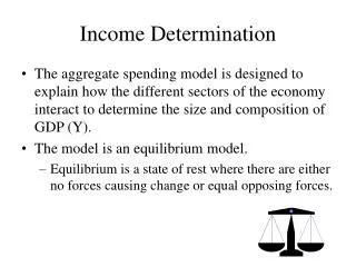
1. Income Determination • The aggregate spending model is designed to explain how the different sectors of the economy interact to determine the size and composition of GDP (Y). • The model is an equilibrium model. • Equilibrium is a state of rest where there are either no forces causing change or equal opposing forces.

2. Equilibrium • Equilibrium is achieved in the model when aggregate spending or expenditures just equal aggregate supply or output. • Aggregate expenditures = Aggregate Supply AE AS

3. Aggregate Expenditures • Aggregate expenditures are comprised of all spending done in the economy during a given period of time. • Aggregate expenditures are the sum of consumption spending by the household sector, investment spending by businesses, government spending by all levels of government, and net exports. • AE = C + I + G + (X-M)

4. Aggregate Supply • Aggregate supply is GDP. • It is all final goods and services produced during a given period of time. • AS = GDP or Y • We will assume for now that aggregate supply is perfectly responsive to spending. • Whenever spending changes, aggregate supply changes by an equal amount. • This is an example of a simplifying assumption. We use it to eliminate supply-side problems so we can concentrate on the demand-side of the model, aggregate spending.

5. Aggregate Supply AE AS According to the circular flow diagram and the NIPA, GDP measured from the spending side equals GDP measured from the income side. We use this relationship to draw the AS line. Note that at point E, the distance 0B=0D=ED. Every point on the AS line represents some amount of GDP. B E 0 D Y

6. Aggregate Supply • We depict aggregate supply graphically with a ray from the origin. • Every point on the ray represents GDP measured either from the expenditure side or from the income side. • GDP measured from the expenditure side is on the vertical axis. • GDP measured from the income side is on the horizontal axis. • The AS line in this model NEVER moves.

7. Aggregate Expenditures

8. Consumption Spending • Consumption is defined as all spending done by the household sector on durables, non-durables, and services. • Consumption is assumed to be determined primarily by disposable income (Yd), but it also may be affected by taxes, changes in the price level, and real wealth. • Consumption spending is assumed to obey the absolute income hypothesis.

9. Absolute Income Hypothesis • The absolute income hypothesis says that consumption is directly related to income. • As income rises, consumption rises but by a smaller amount. This means we can write: • C = a0 + bYd • a0 is subsistence consumption. When Yd = 0, some positive consumption still occurs. • The coefficient b is the marginal propensity to consume. It tells us by how much consumption changes when disposable income changes.

10. Consumption Function AE= C Consumption According to the absolute income hypothesis, consumption spending is directly related to disposable income. The intercept of the consumption function, a0, represents subsistence consumption. The slope of the consumption function, /\C//\Y, is called the marginal propensity to consume. The MPC shows by how much consumption changes as income changes. /\C /\Y a0 0 Y

11. Practice • Define the marginal propensity to consume. • What is the MPC when a change in income of 1000 causes a change in consumption of 900? What if a change in income of 1000 caused a change in consumption of 500? • By how much and in what direction will consumption change given the following: • Income rises by $100 and the MPC is 0.8 • Income falls by $250 and the MPC is 0.75 • Income rises by $400 and the MPC is 0.9

12. Saving • Saving is defined as all saving done by the household sector. • Saving is assumed to be determined primarily by disposable income (Yd), but it also may be affected by taxes and real wealth.

13. Saving • Saving is directly related to disposable income. • S = -a0 + (1-b)Yd • -a0 is subsistence saving. When Yd = 0, and consumption is positive, saving must be negative. • (1-b) is the marginal propensity to save, MPS. It tells us by how much saving changes when disposable income changes.

14. Practice • Given the following, fill in the blanks • Yd Consumption Saving MPC MPS • 5000 4000 • 4000 3200 • 3000 2400 • 2000 1600 • Yd = Disposable income

15. Consumption in the AE/AS Model • Changes in any of the variables that determine consumption spending will cause the consumption line to shift. • Increases in consumption shift C up • Consumption rises when taxes fall, real wealth rises, and the price level falls. • Decreases in consumption shift C down • Consumption falls when taxes rise, real wealth falls, and the price level rises.

16. Consumption Spending and Taxes • Taxes are imposed by the government to pay for government supplied goods and services. • Taxes affect consumption because they change disposable income. • Disposable income is defined as personal income minus personal taxes. It is income after taxes. • The process is as follows: • A change in taxes causes a change in disposable income which causes a change in consumption.

17. Consumption and Taxes • A change in taxes causes an opposite change in consumption. • Increases in taxes decrease disposable income, causing peopleto decrease consumption and/or saving. • Decreases in taxes increase disposable income, causing people to increase consumption and/or saving. • /\Taxes /\Yd /\C

18. Consumption, Saving, and Taxes • The amounts by which people change consumption or saving depend on the marginal propensity to consume and the marginal propensity to save. • If taxes decrease by $100 when the MPC is 0.8 and the MPS is 0.2, consumption spending rises by $80 and saving rises by $20. • If taxes increase by $100 when the MPC is 0.8 and the MPS is 0.2, consumption spending falls by $80 and saving falls by $20.

19. Practice • By how much and in what direction will consumption change given the following: • Taxes rise by $300 and the MPC is 0.9 • Taxes fall by $250 and the MPC is 0.8 • Taxes rise by $100 and the MPC is 0.75 • Taxes fall by $1.00 and the MPC is 0.6 • Describe the relationship between taxes and consumption spending.

20. Consumption and Taxes • A change in taxes changes consumption by an amount equal to: /\C = -(/\Tax times MPC). • Note the minus sign reflecting the inverse relationship between consumption and taxes. • Taxes are an exogenous variable (determined outside the model). Therefore, changes in taxes cause the consumption line to shift. • Increases in taxes shift consumption down. • Decreases in taxes shift consumption up.

21. Consumption and Taxes AE= C C2 A change in taxes shifts the consumption function by the amount -(/\Tx x MPC). An increase in taxes shifts the line down from C1 to C0. A decrease in taxes shifts the line up from C1 to C2. Taxes down C1 C0 -(/\Tx x MPC) Taxes up a2 a1 a0 0 Y

22. Consumption and Wealth • Real wealth is the real net value of all the assets that a person owns. • Consumption is directly related to real wealth. • Other things remaining the same, more real wealth permits more consumption. • Increases in real wealth shift the consumption line up. • Decreases in real wealth shift the consumption line down.

23. Consumption and Wealth AE= C C3 C2 An increase in real wealth shifts the consumption line up from C2 to C3. A decrease in real wealth shifts the consumption line down from C2 to C1. C1 Increase in wealth Decrease in wealth a2 a1 a0 0 Y

24. Consumption and the Price Level • The purchasing power of any money fixed asset declines as the price level rises and rises as the price level declines. • Consumption is negatively related to changes in the price level. • Other things remaining the same, • Increases in the price level decrease purchasing power and shift the consumption line down. • Decreases in the price level increase purchasing power and shift the consumption line up.

25. Consumption and the Price Level AE= C C3 C2 A decrease in the price level shifts the consumption line up from C2 to C3. An increase in the price level shifts the consumption line down from C2 to C1. C1 Decrease in prices Increase in prices a2 a1 a0 0 Y

26. Practice • How will the following event affect real consumption spending? What effect will they have on the consumption function? • A rise in the general price level • A rise in the stock market • People believe that a recession is imminent • Taxes are increased • Interest rates fall • People save more for the future

27. Investment • Investment is defined as all spending done by the business sector on plant, equipment, and inventories. • An important determinant of investment spending is the rate of interest. • There is a negative relationship between investment and the rate of interest. • As interest rates rise, investment falls. • As interest rates fall, investment rises.

28. Interest Rates and Investment • The negative relationship between interest rates and investment exists because firms must either borrow or generate their own funds to invest. • As a result, firms are willing to invest in only those projects that pay a return in excess of the borrowing cost or rate of interest paid. • When rates are high, few projects are sufficiently profitable, but as rates fall, more and more projects become profitable.

29. Investment and the Rate of Interest interest rate At i2, the higher rate of interest, investment equals I1. Only a few projects are profitable at this high level. At i1, the lower rate of interest, investment equals I2. As the rate of interest falls, more projects become profitable. i2 i1 I I1 I2 0 Investment

30. Putting Investment in the Model • Investment enters the model as a lump sum; i.e., it does not vary with income (Y). • This is another example of a simplifying assumption. • It means that investment spending will be the same amount at every level of GDP.

31. Investment in the AE/AS Model AE= C I Investment is drawn as a parallel line above consumption, reflecting the assumption that investment enters the model as a lump-sum. The distance between C and C+I represents lump-sum investment. At Y1, consumption equals the line segments Y1B, consumption plus investment is Y1A, and investment is AB. C+I A C B 0 Y Y1

32. Investment in the AE/AS Model • Changes in any of the variables that determine investment spending will cause the investment line and, therefore, the aggregate expenditure line to shift. • Increases in investment shift I and AE up • Investment rises when interest rates fall, optimism rises, taxes fall, and technology changes. • Decreases in investment shift I and AE down • Investment falls when interest rates rise, optimism falls, taxes rise, and technology changes.

33. Investment Determinants • Expectations about the future affect investment directly. • Optimism about future earnings tends to increase investment spending, while pessimism about future earnings tends to decrease investment spending. • Taxes affect investment negatively. • Increases in taxes diminish profits and tend to decrease investment. • Decreases in taxes increase profits and tend to increase investment.

34. Investment Determinants • Changes in technology that improve the productivity of capital tend to increase investment spending. • However, when technology is changing very fast, there may be a lag before businesses invest in the new technology. Why?

35. Investment in the AE/AS Model AE= C I C + I2 = AE2 C + I1 = AE1 An increase in investment spending from I1 to I2 shifts aggregate expenditures from AE1 to AE2. A decrease in investment spending from I2 to I1 shifts aggregate expenditures from AE2 to AE1. 0 Y

36. Practice • What are the components of investment spending in the national income accounts? • Explain what happens to investment spending and the investment schedule when the following occur • interest rates rise by 1% • profit expectations fall suddenly • business taxes on capital investment increase • new technology becomes available • people expect interest rates to rise next year

37. Government Spending • Government spending is defined as all spending done by all levels of government on goods and services. • Government spending enters the model as a lump-sum. • We invoke this simplifying assumption because there is no consistent relationship between government spending and the level of national income.

38. Government in the AE/AS Model AE= C I G Government spending is drawn as a parallel line above C+I, reflecting the assumption that government spending enters the model as a lump-sum. The distance between C+I and C+I+G represents lump-sum government expenditures. At Y1, consumption equals the line segments Y1B, consumption plus investment is Y1A, consumption plus investment plus government spending is Y1E, investment is AB, and government spending is AE. C+I+G C+I E C A B 0 Y1 Y

39. Government in the AE/AS Model • Changes in government spending cause the government line and, therefore, the aggregate expenditure line to shift. • Increases in government spending shift G and AE up • Decreases in government spending shift G and AE down

40. Government in the AE/AS Model AE= C I G C+I+G3 = AE3 C+I+G2 = AE2 C+I+G1 = AE1 An increase in government spending from G2 to G3 shifts aggregate expenditures from AE2 to AE3. A decrease in government spending from G2 to G1 shifts aggregate expenditures from AE2 to AE1. 0 Y

41. Practice • How will the following events affect the aggregate expenditure line and national income? Why? • An increase in consumer optimism • A decrease in taxes paid by consumers • A rise in the general price level • A rise in the stock market • An increase in government spending • Real wealth increases • Interest rates decline

42. Net Exports • Net exports are the difference between the goods and we produce for the rest of the world and the goods and services they produce for us. • Net exports equal exports minus imports • NX= (X- M)

43. Determinants of Net Exports • Exports • Income in the rest of the world • As income in the rest of the world increases (decreases), they buy more (less) from us. • Relative prices • As our prices fall (rise) relative to prices in the rest of the world, they buy more (less) from us. • Exchange rate • As our currency appreciates (depreciates) relative to other currencies, they buy less (more) from us.

44. Determinants of Net Exports • Imports • Income at home in the domestic economy • As domestic income increases (decreases), we buy more (less) from abroad. • Relative prices • As our prices fall (rise) relative to prices in the rest of the world, we buy less (more) from abroad. • Exchange rate • As our currency appreciates (depreciates) relative to other currencies, we buy more (less) from abroad.

45. Net Exports in the AE/AS Model Net exports (Xn) is drawn as a parallel line above C+I+G, reflecting the assumption that net exports enter the model as a lump-sum and that exports exceed imports. If imports exceed exports, net exports is drawn as a parallel line below C+I+G. The distance between C+I+G and C+I+G+Xn represents lump-sum net export expenditures. At Y1, consumption equals the line segment Y1A, consumption plus investment is Y1B, consumption plus investment plus government spending is Y1C, and consumption plus investment plus government plus net exports is Y1E. AE= C I G Xn C+I+G+Xn E C+I+G C C+I B C A 0 Y1 Y

46. Net Exports in the AE/AS Model • Changes in net exports cause the net exports line and, therefore, the aggregate expenditure line to shift. • Increases in net exports shift NX and AE up • Decreases in net exports shift NX and AE down

47. Net Exports in the AE/AS Model AE= C I G Xn C+I+G+Xn3 = AE3 C+I+G+Xn2 = AE2 C+I+G+Xn1 = AE1 An increase in net exports NX2 to NX3 shifts aggregate expenditures from AE2 to AE3. A decrease in government spending from NX2 to NX1 shifts aggregate expenditures from AE2 to AE1. 0 Y

48. Equilibrium in the Model • When the model is in equilibrium, all goods and services produced are demanded by the members of the various sectors of the economy. • Aggregate expenditures = Aggregate supply • The equilibrium in this model is stable. • There are forces built into the model that push it towards equilibrium.

49. Stability of Equilibrium AE= C I G At Y equal to Y1, AE > AS by the amount AB. The excess demand is met by an unexpected decrease in inventories. The sudden decrease signals producers to increase production. As production rises, employment and national income rise. AS C AE D E At Y equal to Y2, AE < AS by the amount CD. Insufficient demand leads to an unexpected increase in inventories. The sudden increase signals producers to decrease production. As production falls, employment and national income fall. A B 0 Y1 Y2 Y3 Y At Y2, AE = AS.

50. Practice AE AS C + I + G j C + I h C f g c e p b d n a m Y 0 Y1 Y2 Y3