Download
1 / 71
720 likes | 986 Views
Equation-Free Uncertainty Quantification: Applications to Stochastic Chemical Reactions and Biological Oscillators. Yu Zou and Ioannis G. Kevrekidis Department of Chemical Engineering and PACM Princeton University Collaborators: Sung-Joon Moon 1 , Katherine A. Bold 1 , Michael A. Henson 2

E N D
Equation-Free Uncertainty Quantification: Applications to Stochastic Chemical Reactions and Biological Oscillators Yu Zou and Ioannis G. Kevrekidis Department of Chemical Engineering and PACM Princeton University Collaborators: Sung-Joon Moon1 , Katherine A. Bold1 , Michael A. Henson2 1 Dept. of Che. Engr. and PACM, Princeton University 2 Department of Chemical Engineering University of Massachusetts, Amherst United Technologies Research Center, East Hartford, CT August 21, 2006
Background for Uncertainty Quantification Fundamentals of Polynomial Chaos Stochastic Galerkin Method Equation-Free Uncertainty Quantification (EF UQ) EF UQ in Stochastic Catalytic Reactions EF UQ in Yeast Glycolytic Oscillations EF UQ in Kuramoto Coupled Oscillators Conclusions Outline
Uncertain Phenomena in science and engineering * Inherent Uncertainty: Uncertainty Principle of quantum mechanics, Kinetic theory of gas, … * Uncertainty due to lack of knowledge: randomness of BC, IC and parameters in a mathematical model, measurement errors associated with an inaccurate instrument, … Scopes of application * Estimate and predict propagation of probabilities for model variables: chemical reactants, biological oscillators, stock and bond values, structural random vibration,… * Design and decision making in risk management: optimal selection of parameters in a manufacturing process, assessment of an investment to achieve maximum profit,... * Evaluate and update model predictions via experimental data: validate accuracy of a stochastic model based on experiment, data assimilation, … Modeling Techniques * Sampling methods (non-intrusive): Monte Carlo sampling, Quasi Monte Carlo, Latin Hypercube Sampling, Quadrature/Cubature rules * Non-sampling methods (intrusive) : perturbation methods, higher-order moment analysis, stochastic Galerkin method Background for Uncertainty Quantification
Fundamentals of Polynomial Chaos Polynomial Chaos: Orthogonal polynomials of independent random variables <Ψi,Ψj>=0 if i≠j, with Spectral expansion (Ghanem and Spanos, 1991) aj’s are called PC coefficients. Notes Selection of Ψj is dependent on the probability measure or distribution of , e.g., (Wiener-Askey Scheme by Xiu and Karniadarkis, 2002) if is a Gaussian measure, then {Ψj}are Hermite polynomials; if is a Lesbeque measure, then {Ψj}are Legendre polynomials.
Stochastic Galerkin (PC expansion) Method(Ghanem and Spanos, 1991) Preliminary Formulation * Model: e.g., ODE * Represent the input in terms of expansion of independent r.v.’s (KL, SVD, POD): e.g., time-dependent parameter * Represent the response in terms of the truncated PC expansion * The solution process involves solving for the PC coefficients αj(t), j=1,2,…,P Model Input: random IC, BC, parameters Response: Solution
Stochastic Galerkin Method Solution technique: Galerkin projection resulting in coupled ODE’s for αj(t), where Advantages and weakness * PC expansion has exponential convergence rate * Model reduction * Free of moment closure problems * Correlation between parameters and solutions ? The coupled ODE’s of PC coefficients may not be obtained explicitly
Equation-free Uncertainty Quantification Microsimulation Restriction Coarse time-stepper (Kevrekidis et al., 2003, 2004) * Lifting (MC, quadrature/cubature): * Microsimulation: * Restriction: For Monte Carlo sampling, For quadrature/cubature-points sampling, is the weight associated with each sampling point. Lifting
Projective Integration (Kevrekidis et al., 2003, 2004) Δts(≥trelaxation+hopt) Δtc (adaptive stepsize control) Fixed-point Computation(Kevrekidis et al., 2003, 2004) α=ΦT(α) • Newton’s Method • Newton-Krylov GMRES • (Kelly, 1995) Lifting Restriction
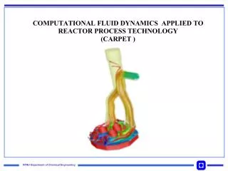
A (CO) +1/2 B2 (O2) → AB(CO2) vacancy CO O2 CO2 : random parameter set Stochastic Catalytic Reactions + F(Θ) ?
Equation Free: Quantities estimated on demand (Kevrekidis et al., 2003, 2004) θ(ξ,t):mean coverages of reactants in catalytic reactions A (CO) +1/2 B2 (O2) → AB(CO2) lifting restriction NA=int(NtotθA)+1 with pA1 int(NtotθA) with pA0 The same to NB θA=<NA>/Ntot θB=<NB>/Ntot NA(t), NB(t), N*(t) NA(t+Δt), NB(t+Δt), N*(t+Δt) Stochastic catalytic reactions: A three-level EF UQ Time-stepper Θ(t+Δt) Θ(t) lifting restriction micro-simulation θ(ξ,t) x θ(ξ,t+Δt) Gillespie Gillespie Algorithm p1 reaction time
Random Steady-state Computation T Number of sites Number of sites lifting restriction ΦT Mean coverages Mean coverages lifting restriction gPC coefficients gPC coefficients Stochasic catalytic reactions Projective Integration Δtf Number of sites Number of sites Number of sites Number of sites Number of sites lifting restriction restriction restriction lifting Mean coverages Mean coverages Mean coverages Mean coverages Mean coverages lifting lifting restriction restriction restriction integrate gPC coefficients gPC coefficients gPC coefficients gPC coefficients gPC coefficients Δts(≥trelaxation+hopt) Δtcc(adaptive stepsize control) Θ=ΦT(Θ)
Stochastic catalytic reactions Projective Integration α=1.6, γ= 0.04, kr=4, β=6.0+0.25ξ, ξ~U[-1,1] gPC coefficients computed by ensemble average Number of gPC coefficients: 12 NeofθA, θBandθ*:40,000 Neof NA, NB and N*: 1,000 Ntotof surface sites: 2002
Stochastic catalytic reactions Projective Integration
Stochastic catalytic reactions Projective Integration α=1.6, γ= 0.04, kr=4, β=6.0+0.25ξ, ξ~U[-1,1] gPC coefficients computed by Gauss-Legendre quadrature Number of gPC coefficients: 12 NeofθA, θBandθ*:200 Neof NA, NB and N*: 1,000 Ntotof surface sites: 2002
Stochastic catalytic reactions α=1.6, γ= 0.04, kr=4, β=6.0+0.25ξ, ξ~U[-1,1] gPC coefficients computed by ensemble average Number of gPC coefficients: 12 NeofθA, θBandθ*:200 Neof NA, NB and N*: 1,000 Ntotof surface sites: 2002
Stochastic catalytic reactions Random Steady-State Computation α=1.6, γ= 0.04, kr=4 β=<β>+0.25ξ,, ξ~U[-1,1] gPC coefficients computed by ensemble average Number of gPC coefficients: 12 NeofθA, θBandθ*:40,000 Neof NA, NB and N*: 1,000 Ntotof surface sites: 2002
Stochastic catalytic reactions Random Steady-State Computation α=1.6, γ= 0.04, kr=4 β=<β>+0.25ξ,, ξ~U[-1,1] gPC coefficients computed by Gauss-Legendre quadrature Number of gPC coefficients: 12 Ne ofθA, θBandθ*:200 Neof NA, NB and N*: 1,000 Ntotof surface sites: 2002
Yeast Glycolytic Oscillations (Wolf and Heinrich, Biochem. J. (2000) 345, p321-334) Notation: A2 - ADP A3 - ATP, A2+A3 = A(const) N1 - NAD+ N2 - NADH, N1+N2 = N(const) S1 - glucose S2 - glyceraldehyde-3-P/ dihydroxyacetone-P S3 - 1,3-bisphospho -glycerate S4 - pyruvate/acetaldehyde S4ex - pyruvate/acetaldehyde ex J0 - influx of glucose J - outflux of pyruvate/ acetaldehyde Reaction rates: v1 = k1S1A3[1+(A3/KI)q]-1 v2 = k2S2N1 v3 = k3S3A2 v4 = k4S4N2 v5 = k5A3 v6 = k6S2N2 v7 = kS4ex Reaction scheme for a single cell glucose J0 cytosol glucose ATP v1 ADP NADH NAD+ glyceraldehyde-3-P/ dihydroxyacetone-P glycerol v6 NAD+ v2 NADH 1,3-bisphospho-glycerate v5 ADP v3 ATP NADH NAD+ pyruvate/acetaldehyde ethanol v4 J v7 pyruvate/acetaldehyde ex external environment
Yeast Glycolytic Oscillations Coupled ODEs for multicellular species concentrations
Yeast Glycolytic Oscillations Heterogeneity of the coupled model: Polynomial Chaos expansion of the solution: Coarse variables: αj and S4ex (25 variables totally) Lifting: Stratified Sampling (1D LH) Fine variables: M – number of cells; M = 1000 (6M+1 variables) Restriction: Minimizing to obtain αj
Yeast Glycolytic Oscillations Full ensemble simulation
Yeast Glycolytic Oscillations Projective integration of PC coefficients S1 S2 S3 S4 A3 A3 N2 t t N2 Time histories of zeroth-order PC coef’s restricted from the full-ensemble simulation A phase map of zeroth-order PC coef’s through projective integration
Yeast Glycolytic Oscillations Limit-cycle computation Poincaré section A3 fixed point ___ limit cycle in the space of PC coefficients xxx restricted PC coefficients of a limit cycle of the full-ensemble simulation limit cycle Poincaré section: In the space of coarse variables, zeroth-order PC coef. of N2 is constant In the space of fine variables, N2 of a single cell is constant N2 Phase maps of zeroth-order PC coef’s through limit-cycle computation
Yeast Glycolytic Oscillations Flow map T – period of the limit cycle Stability of limit cycles imaginary x - PC coefficients o - full-ensemble simulation real Eigenvalues of Jacobians of the flow maps in the coarse and fine variable spaces
Yeast Glycolytic Oscillations Different liftings
Yeast Glycolytic Oscillations Different liftings
Yeast Glycolytic Oscillations Free oscillator N2 of the free cell (CPI) Zeroth-orderPC coefficient of N2 (CPI)
Kuramoto coupled oscillators Lifting: Restriction:
Conclusions and remarks • EF UQ is applied to stochastic dynamical systems with a single • random parameter. • The EF UQ may be extended to include three levels (scales) for • stochastic catalytic reactions. An example with a simple model • is shown. • Possible extensions to models with multiple random parameters • or driven by stochastic processes. References Zou, Y., and Kevrekidis, I.G., Equation-Free Uncertainty Quantification on heterogeneous catalytic reactions, in preparation, available at http://arnold.princeton.edu/~yzou/ Bold, K.A., Zou, Y., Kevrekidis, I.G., and Henson, M.A., Efficient simulation of coupled biological oscillators through Equation-Free Uncertainty Quantification, in preparation, available at http://arnold.princeton.edu/~yzou
Hybrid QMOM-MC Computation on Particle Coagulation and Sintering Processes Yu Zou, Ioannis G. Kevrekidis Department of Chemical Engineering and PACM Princeton University Rodney O. Fox Department of Chemical and Biological Engineering Iowa State University
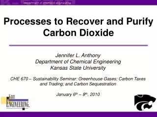
Introduction to particle coagulation and sintering processes SiO2 nanoparticle http://www.nano.fraunhofer.de/de/ institute/kompetenz_izm_cit.html polymer www.msm.cam.ac.uk dust cells www.bloodlines.stemcells.com particle coagulation http://www.bath.ac.uk/~chsscp/group/ particle sintering
Hybrid Univariate QMOM-CNMC Simulations Δtκ Δtκ Δtκ Δtκ p ~ U(0,1) w1 w2 w3 v1, w1 ; v2, w2 ; v3, w3 Product difference algorithm or quadrature-finding subroutines orthog & zrhqr M0 , M1/3 , M2/3 , M1 , M4/3 , M5/3 M0 , M1/3 , M2/3 , M1 , M4/3 , M5/3
Numerical Results Δtd- Δtr- Δte 0.05-0.05-0.4 MC moments Hybrid QMOM-MC time CPU time (sec) Δte
Numerical Results Δtd- Δtr- Δte 0.05-0.05-0.2 MC moments Hybrid QMOM-MC time CPU time (sec) Δte
Numerical Results Δtd- Δtr- Δte 0.05-0.05-0.1 MC MC moments Hybrid QMOM-MC Hybrid QMOM-MC time CPU time (sec) Δte
Numerical Results QMOM self-preserving moments Hybrid QMOM-MC time Δtd- Δtr- Δte 0.05-0.05-0.4
Numerical Results QMOM self-preserving moments Hybrid QMOM-MC time Δtd- Δtr- Δte 0.05-0.05-0.2
Numerical Results QMOM self-preserving moments Hybrid QMOM-MC time Δtd- Δtr- Δte 0.05-0.05-0.1
Hybrid Bivariate QMOM-CNMC Simulations Δtκ Δtκ p ~ U(0,1) w1 … w12 vk, ak, wk k=1,2, …, 12 Minimizing surface area restructuring through the Conjugate Gradient method Mi/3,j/3 i,j=0,1,…,5 Mi/3,j/3 i,j=0,1,…,5
Numerical results Δtd- Δtr- Δte 0.05-0.05-0.2 MC Hybrid QMOM-MC
Numerical results Δtd- Δtr- Δte 0.05-0.05-0.2 QMOM Hybrid QMOM-MC
Numerical results Δtd- Δtr- Δte 0.05-0.05-0.1 MC Hybrid QMOM-MC
Numerical results Δtd- Δtr- Δte 0.05-0.05-0.1 QMOM Hybrid QMOM-MC
Multiscale Analysis on Re-entrant Production Lines:An Equation-Free Approach Yu Zou, Ioannis G. Kevrekidis Department of Chemical Engineering and PACM Princeton University Dieter Armbruster Department of Mathematics, Arizona State University Institute of Industrial Engineers Annual Conference and Exposition Orlando, Florida May 20-24, 2006
Results of Coarse Projective Integration (cont’d) WIP Δtf=0.01s Δth=0.01s Δtc=0.1s time