Summary Statistics/Simple Graphs in SAS/EXCEL/JMP
150 likes | 299 Views
Summary Statistics/Simple Graphs in SAS/EXCEL/JMP. Setting up Program in SAS. In a CIRCA Lab (or maybe in your Department): START -> Programs -> SAS -> (Whatever Version) Three primary Windows will appear (ignore Explorer) :

Summary Statistics/Simple Graphs in SAS/EXCEL/JMP
E N D
Presentation Transcript
Setting up Program in SAS • In a CIRCA Lab (or maybe in your Department): • START -> Programs -> SAS -> (Whatever Version) • Three primary Windows will appear (ignore Explorer): • Editor - This is a standard editor where you will type in or download the commands that constitute your program • Log - This is where the information regarding the running of a program appears. It also will give error messages • Output - Gives results of SAS program (hopefully) • Enter a program in the Editor, then save it (filename.sas), then run it by clicking on Submit (person running image) • Text results will appear in the Output and can be save to a text (List) file and should be named (fulename.lst). Be sure to fully specify the .lst extension or it can overwrite program. • Graphics output can be Copied and Pasted into word processors
Writing a SAS Program • Statements end with semi-colons and can be more than one line long. • OPTIONS Statements can be used for many things, most importantly to frame the page dimensions. • DATA steps are where data are entered (or external datasets are targeted from), variable names assigned, and any new variables created. • Internal datasets are included in program • External datasets are accessed using an INFILE statement • PROC Steps are procedures that act on variables defined or created in DATA steps.
Basic Form of a SAS Program Options ps=54 ls=80; /* frames page to approx. 8.5x11 */ data one; /* This dataset will be called “one” */ input y group; /* Each line will contain two variables on a unit */ datalines; /* The data begins on the next line */ 52 1 73 1 46 2 28 2 ; /* End of data on previous line */ run; proc print; /* Prints dataset */ proc univariate; var y; /* Full-blown summary of variable y */ proc means; class group; var y; /* Mean, SD, min, max of y, for each group */ proc gplot; plot y*group; /* Scatterplot of y versus group */ proc boxplot; plot y*group; /* Side-by-side boxplots of y by group */ quit; /* Ends Program */
Using EXCEL for Summary Statistics • Data Analysis ToolPack has a Descriptive Statistics option which will compute many summary statistics • Many statistical options also available. See Some Useful EXCEL Functions on class website • When obtaining summaries for multiple groups, it’s helpful to create a separate column for each group and copy summary commands across columns
Drawing Boxplots in EXCEL (I) • Step 1: Place data for the various groups in different columns (say A,B,C if there are 3 groups) • Step 2: Obtain the five number summary for each column. • q1: =percentile(range,0.25) • min: =min(range) • median: =percentile(range,0.5) • max: =max(range) • q3: =percentile(range,0.75) • Step 3: Create a table containing these results (using numbers!)
Drawing Boxplots in EXCEL (II) • In Excel 97/2000/2003: • Highlight whole table, including numbers and labels, select Chart Wizard • Choose Line Chart • At step 2, choose Plot by Rows (Columns is default) • On each data series, right-click, and use Format Data Series and remove connecting Lines by selecting None • Right-click on any data series, use Format Data Series, then Options tab and click on switches for High-Low lines and Up-Down Bars • There will not be a line at median, but will be point. Experiment with colors
Example: Impulse Rates of 5 Mollusc Species Original Plot Plot After Removing Lines
Obtaining Plots in EXCEL • Enter data representing the variable on the horizontal axis in the left-most column in the field to be used for data in plot. • Enter data representing the variable(s) on the vertical axis in columns directly to the right-hand side of the column containing the variable to be plotted on the horizontal axis • Click on Chart Wizard, then XY(Scatter), then choose the desired style (points, smoothed lines, jagged lines, etc). Follow steps on dialog box. You can change scales on final graph by right-clicking on the X- and Y-axes and selecting scale. Many other options exist to improve plot quality
Example - Tombstone Weathering Scatterplot • X=100-Year Mean SO2 Concentration of City (ug/m3) • Y=Mean Tombstone Surface Recession Rate (mm/100yr)
Example - Interaction Plot of Means • Response: Seed Weight (Means of samples of size 6) • Factor A: # of fruits on truss (1,2,…,11) • Factor B: Position of Truss on plant (Low/High) • Goal: Plot Mean versus Factor A w/ separate lines for levels of B
Importing Text Data into JMP • Open JMP • Select File Open Files of Type: Text Import Preview • Select Fixed Width • Click off Table Contains Column Headers • Assign Names to Variables • Click Specify Fields • Highlight the the full field for each variable and click Set Field for each variable (Every “column” should be in exactly one field). Click OK when done. (Alternatively you can directly specify the numbers of columns based on data description file) • Click Apply Settings, then OK
Summarizing a Single Variable in JMP • Enter or Import the data in JMP • Select Analyze Distribution • Select variable(s) to be summarized and click on Y,Columns • If you want these separate for different levels of grouping variable(s), select the variable(s) and click on By • Click OK • Summary Stats, Outlier boxplot, and horizontal barchart are printed. Click on red arrows for more options • Copy and Paste can put output in word processor
Side-by-Side Boxplots in JMP • Enter or Import Data into JMP • Make any factor variables nominal by clicking on box next to variable names in Columns box of data editor window • Select Analyze Fit Y by X • Click on Response Variable(s), then Y,Response • Click on (nominal or ordinal) Factor variable(s), then X,Factor • Click OK (This gives a scatterplot) • Click on Red Arrow in Oneway Analysis box, and select Quantiles (This gives side-by-side boxplots) • Copy and Paste into word processor