10. Convolution-based Edge Detection
10. Convolution-based Edge Detection. edge detection computer vision 의 제일 중요한 연산 edge 물체의 경계점 ( boundary of objects) abrupt intensity change ( 급격한 명암 변화) 지점 다양한 edge detection 연산자 1 차 미분에 기반 Roberts Sobel 등 2차 미분에 기반 Laplacian 응용에 따라 요구 다름 아직 미해결 문제 인간 시각은 응용에 adaptive 하게 작동.

10. Convolution-based Edge Detection
E N D
Presentation Transcript
10. Convolution-based Edge Detection • edge detection • computer vision의 제일 중요한 연산 • edge • 물체의 경계점 (boundary of objects) • abrupt intensity change (급격한 명암 변화) 지점 • 다양한 edge detection 연산자 • 1차 미분에 기반 • Roberts • Sobel 등 • 2차 미분에 기반 • Laplacian • 응용에 따라 요구 다름 • 아직 미해결 문제 • 인간 시각은 응용에 adaptive하게 작동
10.1 Laplacian Filter • Laplacian operator • P.S. Laplace (French mathematician, 1749-1827) • Laplacian • 2f(x,y) = 2f/ x2 + 2f/ y2 (함수 f의 2ndorder partial derivative) • intensity 변화 없는 경우 Laplacian은 0 • 즉, edge 아닌 곳에서는 0, edge 에서 (즉, intensity 변화) 반응) • discrete image에서 approximation • 2f(x,y)=4f[x][y]-f[x-1][y]-f[x+1][y]-f[x][y-1]-f[x][y+1] • 즉, Laplacian kernel (요소합은 0) 0 -1 0 -1 4 -1 0 -1 0
10.1 Laplacian Filter • Laplacian 이용한 edge detection (1) Laplacian operator 적용 후 thresholding • 예) 수직 edge 가진 8*8 image 33335555 33335555 0 0 –2 2 0 0 0 0 0 1 0 0 33335555 0 0 –2 2 0 0 0 0 0 1 0 0 33335555 0 0 –2 2 0 0 0 0 0 1 0 0 33335555 0 0 –2 2 0 0 0 0 0 1 0 0 33335555 0 0 –2 2 0 0 0 0 0 1 0 0 33335555 0 0 –2 2 0 0 0 0 0 1 0 0 33335555 Laplacian 적용 Thresholding (T=1)
10.1 Laplacian Filter • Laplacian 이용한 edge detection (2) Laplacian operator 적용 후 zero crosssing 탐지 • 예) 수직 edge 가진 8*8 image 33335555 33335555 0 0 –2 2 0 0 0 0 0 1 0 0 33335555 0 0 –2 2 0 0 0 0 0 1 0 0 33335555 0 0 –2 2 0 0 0 0 0 1 0 0 33335555 0 0 –2 2 0 0 0 0 0 1 0 0 33335555 0 0 –2 2 0 0 0 0 0 1 0 0 33335555 0 0 –2 2 0 0 0 0 0 1 0 0 33335555 Laplacian 적용 zero-crossing
10.1 Laplacian Filter • Laplacian edge detector • 2차미분 연산자 • edge 방향 정보 없음 • noise 많이 발생 • LoG operator • noise 줄이기 위한 목적 • LoG operator 모양 (Mexican hat kernel): Figure 10-5 • 실제 구현에서는 • Gaussian filter 적용 후 Laplacian 적용 • 3*3 kernel 경우 1 2 1 0 -1 0 2 4 2 * 1/16 -1 4 -1 1 2 1 0 -1 0 Gaussian Laplacian • 적용 예: Figure 10-3
10.2 Robert’s operator • gradient (1차미분)기반 operators • Roberts • Sobel • Prewitt • gradient • f(x,y) = (f/x, f/y) • f/x: x 방향 edge 성분 • f/y: y 방향 edge 성분 • digital space • f/x = f[x][y] – f[x+1][y+1] 0 1 0 0 0 –1 0 0 0 • f/y = f[x+1][y] – f[x][y+1] 0 0 1 0 -1 0 0 0 0
10.2 Robert’s operator • edge magnitude (에지 강도) • |f(x,y)| = ((f/x)2 + (f/y)2)1/2 • digital space • ((f[x][y] – f[x+1][y+1])2 + (f[x+1][y] – f[x][y+1])2)1/2 • Roberts 적용 • Figure 10.6 • Roberts 적용 후 thresholding • Figure 10.7 • UNHE 적용 후 • Roberts 적용
10.3 Sobel operator • Sobel operator • f/x 1 0 -1 2 0 -2 1 0 -1 • f/y -1 -2 -1 0 0 0 1 2 1
10.3 Sobel operator • Sobel 적용 • Figure 10.8 • Figure 10-9 • Figure 10-10 • Figure 10-11 • Figure 10-12