OS12B-156

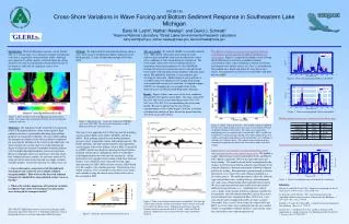
1. OS12B-156 Cross-Shore Variations in Wave Forcing and Bottom Sediment Response in Southeastern Lake Michigan Barry M. Lesht1, Nathan Hawley2, and David J. Schwab2 1Argonne National Laboratory; 2Great Lakes Environmental Research Laboratory barry.lesht@anl.gov, nathan.hawley@noaa.gov, david.schwab@noaa.gov Introduction: The Lake Michigan recurrent coastal “plume” (Fig. 1) is a basin-wide, wave-induced, nearshore resuspension event that is triggered by strong northerly winds. Although most apparent in satellite imagery collected during the spring, similar events also occur during the fall and winter whenever the winds are sufficient for significant surface wave development. Methods: We deployed three instrumented moorings along a cross-shore transect off Muskegon, MI in southeastern Lake Michigan (Fig. 2) from 13 September through 30 October 2000. The wave model: We used the GLERL wave model (Schwab et al., 1984) driven with hourly observations of winds collected from around the study area to estimate the surface wave conditions at each station during the experiment. The wave model, which solves the two-dimensional wave momentum conservation equation, uses the JONSWAP relations between wave momentum and wave height to link wave energy with with peak energy frequency and mean wind speed. We applied the model on a 2 km rectilinear grid covering the entire lake. Model output at each grid point at each hour consists of significant wave height, peak-energy wave period and average wave direction. A companion paper (OS32U-04) comparing the wave model results to the observed waves will be presented Wednesday afternoon. The offshore variation in near-bottom suspended sediment concentration closely matches the offshore distribution of wave energy.Figure 5 is a planar time-depth section showing the distribution of near-bottom suspended sediment concentration (color scale) overlain by a contour of constant near-bottom wave orbital velocity (0.15 m s-1) estimated from the modeled wave height and period by using linear wave theory.Resuspension was observed at stations M19 and M25, but not at M55. Figure 6. Observed and predicted TSM at station M19. Results: Figure 4 shows time series of the basic conditions measured by the tripod at station M25. One large storm (9/21; day 265) and several coastal upwelling events (9/15, 9/25, 10/5; days 259, 269, 279) occurred during the observation period. Because it appears that the near-bottom transmissometer at this station began to foul late in October, we limited our analysis of these data to the period from day 257 (9/13) to day 296 (10/21). Figure 7. Observed and predicted TSM at station M25. Figure 1. Three instances of the Lake Michigan recurrent coastal plume. The images show maximum reflectance observed during the spring of each year. Model parameter values are consistent with sediment type. Figure 2. Episodic Events - Great Lakes Experiment (EEGLE) study area (1998-200). The transect described here is off of Muskegon, MI in the northeast sector.. Figure 5. Isoline (white) of 0.15 m s-1 wave orbital velocity overplotted on time-water depth contour map (color scale) of near-bottom (0.9 mab) suspended sediment concentration. The isoline was calculated by interpolating the wave model results at stations M19, M25, and M55 for each hour to a regular grid representing water depths ranging from 16 m to 60 m and using the grid depth with the interpolated wave conditions to calculate wave orbital velocity. The sediment concentration map was estimated by contouring the half-hourly observations made at the three stations. • Objectives: One important feature of the these resuspension events is the limited offshore extent of the region of high radiance reflectance, presumably indicating sharp offshore gradients in resuspended sediments. Because understanding the transport of materials across these gradients is important for assessing the influence of the events on the whole lake, our observational focus in this study was on determining the degree to which the horizontal suspended sediment gradient reflected depth-dependent gradients in local resuspension. Because companion efforts are underway to develop whole-lake sediment dynamics models, we also were interested in using our observations to develop and test simple sediment transport models. Among the questions we address here are: • Can we determine a consistent set of threshold and entrainment rate values for use in simple sediment transport models? How well can the observed sediment transport be simulated by using modeled surface waves as forcing? • What is the relative importance of horizontal variation in sediment type relative to horizontal variation in the wave forcing in the transport models? The transect was approximately 10-km long and the moorings were located at depths of 16 (M19), 26 (M25), and 56 m (M55). Each mooring included a near-bottom-mounted pressure sensor, temperature sensor, and transmissometer. The deeper moorings also had transmissometers and temperature sensors higher in the water column (10 m at M25, 10 m and 25 m at M55) and the two shallower moorings had near-bottom-mounted current meters, although the meter at station M19 failed approximately one week into the experiment. All the instruments were sampled in burst mode at half-hour intervals. Surface wave conditions were estimated by using either spectrum analysis (M19, M55) or burst statistics (M25) based on 4 Hz samples of the absolute pressure. Near-bottom wave orbital velocities were estimated by using linear wave theory, and verified by using the current meter observations (also 4 Hz) recorded at M25. Largest errors are correlated with northwesterly waves. Simple models can reproduce the important features of the observed near-bottom concentration time series. We applied a simple sediment mass conservation model (Lesht and Hawley, 1987; Hawley and Lesht, 1992) to the data collected at all three stations. The model is based on the assumption that the changes in the local near-bottom sediment concentration result from the differences between entrainment of bottom sediment and loss by settling. Resuspension is parameterized as a linear function of excess shear stress and settling is modeled as a first order process. The model parameters reflect the sediment type (critical shear stress, settling velocity, and entrainment rate) and a non-settling background suspended concentration. We have experimented with other model forms that involve different forcing functions (e.g., combined wave-current stress), limits on the amount of bottom sediment available for resuspension, and with erosion-dependent critical shear stress and entrainment rates (Sanford and Maa, 2001) but it is not clear that the more complicated models are more accurate. Our model (Figs. 6 and 7 show results for stations M19 and M25) uses wave shear stress calculated from the wave model, infinite resuspendable sediment thickness, and constant values for critical shear stress and entrainment rate. Figure 8. Station 25 prediction error and modeled wave direction. References: Hawley, N. and B. M. Lesht, 1992. Sediment resuspension in Lake St. Clair. Limnol. and Oceanogr., 37(8):1720-1737. Lesht, B. M., and N. Hawley, 1987. Near-bottom currents and suspended sediment concentration in southeastern Lake Michigan. J. Great Lakes Res., 13(2):375-386. Sanford, L. P. and J. P.-Y. Maa, 2001. A unified erosion formulation for fine sediments. Mar. Geol., 179:9-23. Schwab, D. J., J. R. Bennett, P. C. Liu, and M. A. Donelan, 1984. Application of a simple numerical wave prediction model to Lake Erie. J. Geophys. Res. 89:3586-3592. Figure 4. Time series of observations made at station M25. Pressure and velocity measurements (shown as horizontal velocity vectors) were made 0.7 m above the bottom (mab). Sediment concentration is based on transmissometer measurements made 0.95 mab (solid) and 10 mab (dashed). Temperatures also are from 0.95 mab (solid) and 10 mab (dashed). _________________ This work was supported by NOAA’s Coastal Ocean Program under Interagency Agreement with the U. S. Department of Energy as part of the Episodic Events: Great Lakes Experiment (EEGLE) project. Figure 3. Schematic representation of instrument array.