Download
1 / 27
280 likes | 460 Views
Probing anisotropic expansion history of the universe with CMBR. Ajit M. Srivastava Institute of Physics Bhubaneswar. Work done with: Ranjita K. Mohapatra, P.S. Saumia. Outline: Basic question posed here: Universe could have expanded

E N D
Probing anisotropic expansion history of the universe with CMBR Ajit M. Srivastava Institute of Physics Bhubaneswar Work done with: Ranjita K. Mohapatra, P.S. Saumia
Outline: • Basic question posed here: Universe could have expanded • anisotropically during some early stage, e.g. during inflation, • subsequently entering isotropic expansion stage • 2. Can we investigate this using CMBR? • 3. In particular, can we distinguish anisotropic initial conditions • for fluctuations from a transient anisotropic expansion stage ? • We propose a simple technique for the shape analysis of • overdensity/underdensity patches • This technique can be useful for other systems such as • domain growth in phase transitions in condensed matter • systems. • This can provide useful direct information on elliptic flow • in relativistic heavy-ion collisions: ongoing work
Isotropy of the universe? Distribution of matter, CMBR fluctuations, indicate general isotropy of the universe at present Possible anisotropy of the universe is extensively investigated: Anomalous multipole alignment: hints of a preferred axis … Statistical isotropy violation: Souradeep’s talk We ask the question about anisotropy in the expansion rate of the universe (at some early stage) Present expansion of the universe appears to be isotropic However: Universe could have expanded anisotropically during some early stage, e.g. during inflation, subsequently entering isotropic expansion stage
Can we put constraints on such an early, transient, stage Of anisotropic expansion using CMBR data ? In, as much as possible, model independent way (not even assuming inflationary stage) The basic idea we follow is that the superhorizon fluctuations in the universe retain their shapes during isotropic expansion stage., while during anisotropic expansion shapes get deformed. Further, deformations are identical for all superhorizon fluctuations. This may not necessarily be true for subhorizon Fluctuations. An analysis of shapes of superhorizon fluctuation patches in CMBR should reveal the information about any early anisotropic Expansion history.
There are other techniques, e.g. Minkowski functionals have been used for shape analysis of CMBR and for large scale structure. For example, for analyzing topological properties of fluctuations There has also been study of the ellipticity of anisotropy Spots of CMBR, and the orientation of such ellipticity. (Gurzadyan et al. arXiv: astro-ph/0503103) This has similarities with our technique, though there are Fundamental differences. However, a general study of shape deformations resulting From an anisotropic expansion history has not been performed
Our analysis is based on the following general picture: Spherical patches always remain spherical isotropic expansion isotropic expansion Spherical patches become ellipsoidal, subsequently they retain their deformed shapes isotropic expansion anisotropic expansion
However, actual CMBR fluctuation patches have no simple Geometrical shapes: 20 deg X 20 deg region at equator for WMAP 7Yr Data (ILC map) How do we detect any shape anisotropy in overdensity patches in such a picture ?
Note: Even with the random shapes, average shape of the fluctuation will be spherical (isotropic) Isotropic expansion will stretch the fluctuations symmetrically. Anisotropic expansion stretches the fluctuations asymmetrically Average shape will become ellipsoidal if the expansion is asymmetric along one direction. For superhorizon fluctuations this shape anisotropy will remain during subsequent isotropic Expansion stages. Important: This shape analysis of CMBR patches can give information about any transient stage of anisotropic expansion, from the Time when fluctuations were created, upto the stage of Last scattering. We will further show that our technique can distinguish between anisotropies resulting from initial conditions from those arising from anisotropic expansion.
We determine shape anisotropies in the following two ways: • By direct analysis of widths of slices of overdensity • patches in x and y (i.e. q and f) directions. • That is: we determine shape anisotropies in real space • Using 2D Fourier transform, and determine anisotropy • in the Fourier space. • This second method has been used in other areas • (metallography) for studying anisotropies. • (Holota and Nemecek, Applied Electronics, 2002, p:88) • They used a digitized image of the material. Then calculate • 2D Fourier transform which is thresholded to levels 0 and 1. • Anisotropy in the Fourier space is determined by the ratio • Of the widths of the histograms in the two directions.
10% deformation 20% deformation 30% deformation Material structures and their spectrum obtained by the 2D Fourier Transform
Ratio of the widths of the two peaks is taken as a measure Of the anisotropy of the pattern in the pictures. We will apply this technique also for analyzing CMBR fluctuations
In our second technique, we study the geometry of fluctuations directly in physical space, in the following manner: We use ILC smoothed WMAP 7Yr map Consider patches of different ΔT intervals on a 20 degree belt along equator (important to get filled patches) Divide the 20 degree belt into 0.05 degree strips along latitude and longitude. This will be most sensitive for anisotropic expansion along z axis compared to x-y plane. Measure X and Y extents of filled patches in these strips and calculate the histogram of the resulting distributions. X and Y histograms should fall on top of each other if the average shape of fluctuations is spherical, i.e. if the expansion (and the initial conditions) were isotropic. Repeat for different orientations of the z axis, to detect anisotropy along any other direction. (Difficulties due to pixel arrangements in HEALPix)
θ sin θ dΦ
We simulate anisotropic expansion along Z -axis by stretching the CMBR temperature fluctuations along Y-axis by a given factor (equatorial belt is most sensitive for anisotropic expansion along the Z-axis) • We find that the X and Y histograms don’t overlap • Using different stretching factors, and determining difference between the histograms, one can put constraints on the anisotropic expansion of the universe. • We also simulate a distribution of spherical patches for which the histograms are plotted as above. Anisotropies are introduced using stretched (ellipsoidal) patches. • This allows us to distinguish the effects of anisotropic initial conditions from the effects of anisotropic expansion history
Histograms forf and q Directions for original CMBR data (20 degree belt around equator). Note: complete overlap of the plots, also note peak near 1 degree CMBR data stretched By a factor 2 along q Direction. Plots don’t Overlap. Note: shift in the peak for q plot to about 2 degree
2D Fourier transform Same patches (original data, above, and stretched data, below) analyzed using Fourier transform technique. 2D Fourier transform
Histograms of the Fourier transforms (using some threshold value for levels 0 and 1). For top, histograms overlap while below they do not.
We now discuss simulated geometrical shapes: A cubic lattice is created where randomly located filled spheres are generated. We use well defined geometric shapes, instead of random shapes, so that anisotropy of the shape can be directly identified and then related to our measures of shape anisotropy. A spherical surface centered at the center of the cube, is constructed and its intersection with the filled spheres is taken as the CMBR map at the surface of last scattering. Subsequent analysis is identical to what is presented earlier for the CMBR data. By changing spherical shapes to ellipsoidal, and/or by making their distribution anisotropic different initial conditions are represented as discussed below
We will discuss following three cases: • Spherical patches, distributed uniformly. This means • fluctuation generation mechanism as well as the universe expansion are isotropic. • In this case, both methods give overlapping plots. • 2. Spherical patches, distributed anisotropically. • This could only happen if fluctuations (of isotropic • shapes) were generated with anisotropic distribution • (possibly due to some biasing field). However, expansion • must be isotropic here otherwise shapes will get deformed. • Here Fourier transform histograms don’t overlap, but • real space histograms still overlap as they are only • sensitive to filled patches
3. A difficult case to distinguish (from anisotropic expansion) is the following: Fluctuations could be anisotropic to begin with, possibly due to some biasing field. Here for both methods plots will not overlap, as both methods will detect anisotropy. However, any biasing field is unlikely to create exact same anisotropy factor (eccentricity) for fluctuations of different length scales. This will imply that fluctuations of different sizes will have different shape anisotropies. With this extra information, we will see that the real space method can distinguish this case from anisotropic expansion. For the Fourier transform method, the difference is not so clear.
Spherical patches: uniform distribution (above) and nonuniform one (below). Note: anisotropic expansion will always lead to ellipsoidal shapes Same plots for Both cases as We only detect Filled patches
Note: Fourier transform method cannot distinguish between anisotropic Expansion from anisotropic distribution (resulting from initial conditions)
Anisotropic shapes with Eccentricity increasing with size of fluctuation Note: both plots have peaks at similar location Distribution of sizes, all With same ellipticity Note: peak for q is shifted due to stretching
Same two cases again. Hard to distinguish from the Fourier transform Technique. Real space plots seem to show qualitative difference.
Constraining the stretch factor S (anisotropic expansion) S = 1.35 S = 1.5 S = 1.3 S = 1.2
Concluding Remarks Thus our technique provides an effective method to detect shape anisotropies in the density distribution which is characteristic signature of any anisotropic expansion in the early universe. It is important to note that this constrains, in an model independent way, any anisotropic expansion, e.g. starting from the inflation to the surface of last scattering. Within angular scales examined by us (20 degree belt), we do not detect any anisotropy in expansion. A rough estimate is less than about 35% anisotropy (by just noting difference between histograms for the stretched data by factor 1.35, where anisotropy can be barely noticed). With PLANCK data one should be able to do shape analysis of Patches with high resolution: Information about shape changes during gravitational collapse of fluctuations, viscosity effects..
This technique of shape analysis (especially in real space) can be very useful for other systems such as in condensed matter physics (in studies of growth of domains during phase transitions). We are applying it to study anisotropic flow (elliptic flow) in relativistic heavy-ion collision experiments by doing shape analysis of energy density/particle multiplicitiy fluctuations. This can give direct information about anisotropic flow