Spreadsheet-Based Decision Support Systems Chapter 5: Charts Overview
300 likes | 319 Views
Learn to create dynamic charts using various chart options with the Chart Wizard in spreadsheets. Customize and locate charts effectively, understand chart types, source data, and chart options. Enhance data visualization for optimal decision-making.

Spreadsheet-Based Decision Support Systems Chapter 5: Charts Overview
E N D
Presentation Transcript
Spreadsheet-Based Decision Support Systems Chapter 5: Charts Prof. Name name@email.com Position (123) 456-7890 University Name
Overview • 5.1 Introduction • 5.2 Creating Charts with Chart Wizard • 5.3 Working with Chart Options • 5.4 Creating Dynamic Charts • 5.5 Summary
Introduction • Creating a chart using the Chart Wizard • Customizing charts using various chart options • Creating dynamic charts
Creating Charts with the Chart Wizard • Charts are used to take data from a table and transform it into a graphical illustration • They are useful for displaying data patterns or results • To create a chart, we will use the Chart Wizard • Insert > Chart from menu • icon from standard toolbar
The Chart Wizard • There are four main steps in using the Chart Wizard: • Step 1: Chart Type • Step 2: Source Data • Step 3: Chart Options • Step 4: Chart Location • Chart Type = bar graph, scattered graph, pie chart, etc • Source Data = data range or various series • Chart Options = title, axes, legend, gridlines, etc • Chart Location = object or chart sheet
Figure 5.1 • Table of data = Number Sold and Revenue Generated from various Car Models • We create two charts: bar graph of Number Sold and pie chart of Revenue Generated
Step 1: Chart Type • Each chart type has a set of chart sub-types. • First we will select Column as our chart type. • We can now choose a sub type that is either a 2D or 3D • Clustered Column • Stacked Column • 100% Stacked Column
Step 2: Source Data • Source Data can be defined by a Data Range or with Series • Data Range is the main data table we initially highlighted to be graphed. • Rows = comparison is made among rows of data from the table • Columns = comparison is made among columns of data from the table
Step 2: Source Data (cont’d) • Series are the rows or columns of data from the table which are being compared. • Series can be • Added • Removed • Named
Step 3: Chart Options • Tabs of the Chart Options step include: • Titles • Axes • Gridlines • Legend • DataLabels • DataTable
Step 3: Chart Options (cont’d) • Titles options include chart, category (X) axis, and value (Y) axis titles
Step 3: Chart Options (cont’d) • Axes options include Category (X) and Value (Y) axes • Automatic = default • Category = any grouping of axes values • Time-scale = dates or time units
Step 3: Chart Options (cont’d) • Gridlines options include Category (X) and Value (Y) axes • Major gridlines • Minor gridlines
Step 3: Chart Options (cont’d) • Legend options include showing or hiding the legend, and placement of the legend
Step 3: Chart Options (cont’d) • DataLabels options include showing or hiding data values and labels
Step 3: Chart Options (cont’d) • DataTable options include showing or hiding the data table
Step 4: Chart Location • The chart can be completed as • A new chart sheet; name is given • An object in a current sheet; name of sheet is selected
Figure 5.6 • From the bar graph we see that the Aco3500 sold the most cars
Figure 5.7 • We repeat the Chart Wizard steps to create the pie chart of Revenue Generated • We see that the Cam3200 generated the most revenue
Working with Chart Options • After creating a chart using the Chart Wizard, we can return to any of the Wizard steps by simply right-clicking on the chart. • The Format Chart Area option also allows us to modify the general patterns, font, and properties of the chart. • Format Plot Area • Format Data Series • Format Axis
Figure 5.9 • Data table shows plant growth based on minerals added or removed from the ground
Figures 5.14 and 5.16 • Create the chart • Chart Options can be used to switch x and y values for better data analysis
Creating Dynamic Charts • A chart is linked directly to the Data Range specified in the Source Data step of the Chart Wizard. • If any points in this range of data are modified, the chart is automatically updated to reflect a new corresponding data point. • There will be three main Excel concepts used to create a dynamic chart: • Defining names • OFFSET function • COUNT function
Dynamic Charts (cont) • Create some range names using the OFFSET and COUNT functions and set the Series of the chart to these dynamic ranges. • =OFFSET(initial_data_location, 0, 0, COUNT(entire_column), 1) • The rows_to_move and columns_to_move parameters are set to 0 because we are only interested in the column in which our reference_cell ( = initial_data_location) is located. • The width is again set to 1, since we are interested only in one column. • The height parameter is found using the COUNT function. • The COUNT function will review the entire column of the relative data and count how many cells have numeric values. • Thus the height of our range becomes dynamic as the amount of numeric values in the column increases.
Figure 5.17 • Months and Units Sold may be dynamic values
Figure 5.18 • The dynamic ranges are created for each column using the OFFSET and COUNT functions
Figure 5.19 • The Series are set using these dynamic ranges
Figure 5.20 • The chart is now dynamic
Summary • Excel Charts allow you to illustrate your data in order to perform better analysis. • There are four basic steps in the Chart Wizard: • Step 1: Select the Chart Type and options. • Step 2: Verify or change the Data Range and define all Series. • Step 3: Determine the Chart Options. • Step 4: Choose the location of the chart. • A chart can be modified after it is created by right-clicking on the chart or different parts of the chart. You can change basic settings as well as formatting. • A dynamic chart can be created using the OFFSET and COUNT functions to create dynamic ranges used as Series in the Source Data.
Additional Links • (place links here)