Download
1 / 55
560 likes | 716 Views
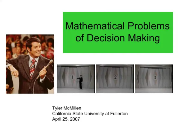
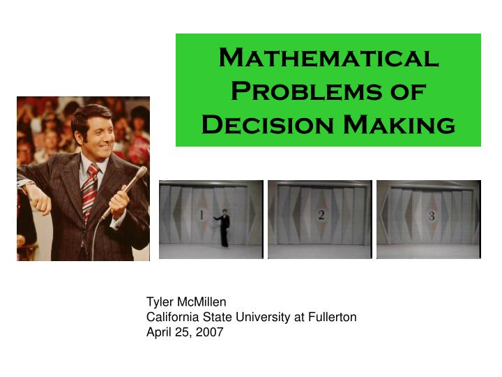
Mathematical Problems of Decision Making. Tyler McMillen California State University at Fullerton April 25, 2007. Questions. How do you choose between multiple alternatives? Is there a “best” way to choose? Is the brain “hard-wired” to choose in the best way? (or not such a good way…).

E N D
Mathematical Problems of Decision Making Tyler McMillen California State University at Fullerton April 25, 2007
Questions How do you choose between multiple alternatives? Is there a “best” way to choose? Is the brain “hard-wired” to choose in the best way? (or not such a good way…)
Overview • Description of problem • Modeling perceptual choice • Hypothesis testing • Decision making • Sequential effects
…or… run … or … fight hit … or … stay pure…or…applied country…or…western door number 1,2 or 3? whose face is that?
lied died lien
lied lien reconstruction
90 or 0 45 or 25 45 or 40
Models of decision making • Hard! Simplest types of decisions only partially understood • Statistical regularities: • Reaction Times (RT), Error Rates (ER), etc. • Hick’s Law: RT ~ log(N) • Loss avoidance • Magic number 7 (plus or minus 2)
Hick’s Law & Information Transmission RT ~ A log(N) + B (up to a point…)
Threshold Crossing dx = a dt + c dW (drift-diffusion equation)
Stochastic Differential Equations (SDEs) (Fokker-Planck equation) Drift-diffusion equation 1-D Ornstein-Uhlenbeck equation
Perceptual model for 2 choices I2 I1 Input Q: Which is larger, I1 or I2? + noise x1 Inhibition: w x2 Neural units Decay: k
Perceptual model for 2 choices Collapse to a line: Dynamics determined by: x = x1 – x2 dx = [(w-k) x + a] dt + c dW (when “balanced”, w = k) dx = adt + c dW Equivalent to SPRT – optimal test! (Best when k=w.) (Can calculate explicitely ER, RT, RR. Behavior of humans, chimps, seems to fit that predicted by the drift-diffusion model. Cf. Ratcliff, et.al.)
no noise noisy x1 correct Dashed - no inhibition or decay Solid - inhibition & decay Inhibition “sharpens” acuity (spreads alternatives)
Neural models of perceptual choice … I1 I2 IM Q: Which is larger, I1, I2, … , IM? Input +noise … Neural units: x1 x2 xM Inhibition Decay
Neural models of perceptual choice Does the model capture observed behavior, e.g., Hick’s Law? Can we show that the model performs optimally? (or not?) Two different kinds of tasks: Free-response (make a decision any time) Interrogation (forced to decide at a given time) What does the model say about the difference in behavior in the two kinds of tasks?
Optimality The optimal decision making algorithm is the one that minimizes the time needed to make the decision (RT) for a given error rate (ER). This is equivalent to maximizing the reward rate (RR), the ratio of the probability of being correct to the time needed to make a decision:
Hypothesis Testing Neyman & Pearson (1933) – optimal tests for fixed sample sizes Wald, Friedman, Wallis, Barnard, Turing (1940’s) – optimizing the sample size in tests between two alternatives Wald, Sobel, Armitage, Lorden, Dragalin, … (1940’s-present) – nearly optimizing tests for more than two alternatives
Testing between M alternatives: H1, H2, … , HM Know: pi(x) = P(x|Hi) (If Hi is true, the density of x’s is pi(x) ) Which is the correct distribution? Suppose we draw 5 samples: Example: 3 hypotheses How confident can we be in our decision? How many trials should we make before we stop?
Drift-diffusion equation: Path: Another way to view the problem. Decision will depend on the “path” of the sum of samples:
Test between two hypotheses H1 and H2: (likelihood ratio) • Fixed Sample Size Tests • If the number N of samples x1,…,xN is fixed, • Neyman-Pearson Lemma (1933) says the best result will be • obtained by taking Value of K determines accuracy.
Test between two hypotheses H1 and H2: (b) Sequential Tests If testing can stop at any time, SPRT gives best result: SPRT: Continue testing until 21 crosses an upper or lower threshold Choose H1 Choose H2 SPRT Optimality Theorem: (Wald) Among all tests with a given bound on the error rate, the SPRT minimizes the expected number of trials Q: Is there a generalization of the SPRT, an “MSPRT,” with the same optimality property?
Test between two hypotheses H1 and H2: As the number of samples increases, SPRT approaches threshold test on drift-diffusion equation (sampling at each instant).
Two Approaches Test between more than two hypotheses: • Continue testing until one hypothesis is preferred to all others. (Use SPRT’s as component tests between the hypotheses.) Sobel-Wald Test on 3 hypotheses (1949) Armitage Test on multiple hypotheses (1950) Simons Test on 3 hypotheses (1967) MSPRT (1990’s) • Continue testing until all but one hypothesis can be rejected. (In the spirit of significance testing, based on generalized likelihood ratios.) Lorden Test (1972) m-SPRTs No optimal test!
Continue testing until pnj or Lj(n) cross threshold, choose the first one that crosses. Note: Both tests reduce to SPRT when M=2 Multi-Sequential Probability Ratio Tests (MSPRT’s) j: prior probability of Hj THEOREM: (Dragalin, Tartakovsky and Veeravalli, 1999) The MSPRT’s are “asymptotically optimal”: As the error rate approaches zero, the expected sample size in the MSPRT’s is bounded by the infimumum over all tests.
MSPRT on 3 alternatives Samples: x1,x2, … red - a blue - b Unequal prior probabilities 1=.8, 2=.15, 3=.05 (biased) Equal prior probabilities (unbiased)
Perceptual model for M>2 choices … I1 I2 IM Input: Q: Which is larger, I1, I2, … , IM? + noise … Neural units: x1 x2 xM Inhibition: w Decay: k (Usher & McClelland, ’01)
Connectionist Model This model has been successful in modeling response time, error rate, etc., statistics, in several cases. Additionally captures loss-avoidance phenomenon. Q: Is it optimal? Can we say anything about what happens when the number of alternatives increases?
Connectionist Model MSPRT b test on : Choose first i that satisfies M=2 model performs the optimal test. What about for M>2?
Absolute and relative tests absolute max-vs-next max-vs-average relative tests perform better (because of noise)
0.6 max-vs-average 0.6 0.1 0.6 max-vs-next Max-vs-next is better (more information), but computationally more expensive.
On , xi threshold crossing is equivalent to the “max vs average” test. Collapse to a Hyperplane Transform on eigenvectors:
Calculating RR For 2 alternatives, can write (backward Kolmogorov) equations for 1st passage time (RT) and error rate (ER) as BVP’s: For M>2 alternatives, backward Kolmogorov equations are drift-diffusion BVP’s on (hyper) triangles: Can be solved explicitely to give expressions for RR as function of parameters. No explicit solution. Solving numerically not easier than Monte Carlo simulations.
4 alternatives Pr(correct) = 0.95 Best: max-vs-next Good: max-vs-ave (same as threshold crossing) Worst: “unbalanced” Balanced (w=k) gives best result. Hick’s Law
Interrogation Protocol Optimal when w=k (magnitude of w,k irrelevant) TI = time to reach a given accuracy Hick’s “type” Law
Interrogation vs. Free Response Time to reach a given accuracy P. (2 choices) Free-response does better – a particular example of the fact that sequential tests perform better than fixed sample size tests – That’s why they were invented!
Sequential effects Cho, et.al. Mechanisms underlying dependencies of performance on stimulus history in a two-alternative forced-choice task. (2002)
Effects of inter-trial delay W. SOMMER, H. LEUTHOLD and E. SOETENS, Covert signs of expectancy in serial reaction time tasks revealed by event-related potentials Perception & Psychophysics 1999, 61 (2), 342-353