Linear Systems
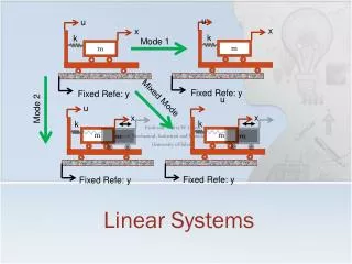
u. x. k. Linear Systems. u. m. x. k. Mode 1. m. Professor Walter W. Olson Department of Mechanical, Industrial and Manufacturing Engineering University of Toledo. Fixed Refe : y. Fixed Refe : y. Mixed Mode. u. u. Mode 2. x. x. k. k. m. m. m. m. Fixed Refe : y.

Linear Systems
E N D
Presentation Transcript
u x k Linear Systems u m x k Mode 1 m Professor Walter W. Olson Department of Mechanical, Industrial and Manufacturing Engineering University of Toledo Fixed Refe: y Fixed Refe: y Mixed Mode u u Mode 2 x x k k m m m m Fixed Refe: y Fixed Refe: y
Outline of Today’s Lecture • Review • System Response • Hypothetical but common 2ne Order System Response • Stability • stable • unstable • marginal or neutral stability • Linear Systems • Functions of Square Matrices • Eigenvalues • Stability • Modes
Hypothetical (but Common Form) 2nd Order System 5 Phase Plots Equilibrim Points Limit Cycles
System Response: Step Input • The time history of a system’s outputs Often called the system path, trajectory or time series { Overshoot Mp Steady State Rise time, tr Transient period=settling time, ts
System Response: Frequency Response • Time history with respect to a sinusoid: Phase Shift, DT Amplitude Ay Amplitude Au Input Sin(t) Period,T Transient Response
Types of Common Responses General form of linear time invariant (LTI) system is expressed: The most general form of the response (the solution) is expressed:
Definition of Stable • A system described the solution (the response) is stable if that system’s response stay arbitrarily near some value, a, for all of time greater than some value, tf.
Hypothetical (but Common Form) 2nd Order System 5 Phase Plots Unstable Stable Marginally Stable
What is a Linear Systems • In order to be Linear, a system f(x) must obey the rules • So why is this important for controls?
Linear Control Systems • If we have two responses known from our system, say, then we also can find the response to the sum of the imput:
Transformations of Linear Systems • Does my system operate any differently is I observe it in a different coordinate system? x1 z2 x2 z1
Transformations of Linear Systems • The only changes are in the variables! For a linear transformation, we want it to be invertible such that we can move from one system to the other. These are known as similarity transformations x1 z2 x2 z1
Functions of Square Matrices • We can perform the following operations with the square matrix A: • Then we can form a polynomial in A: • We have create a function of our matrix which can be shown to to factor as
The Exponential Function of a Square Matrix A • A Taylor series of the exponential function of x is • Thus we can define as the matrix exponential • In Matlab, the comandexpm(A) computes • And we can use this just as we would any other function • For Example, the solution of is and
What Does this mean for a Linear System? • The homogeneous solution is the solution where u(t)=0 • Therefore we can write “a” solution for the system with no input • In Matlab, this solution is displayed with the command initial(A,B,C,D,x0)
>> k = 250000; % Nose wheel spring stiffness N/m kt = 5000000; % Nose wheel tire stiffness in N/m b = 125000; % Nose wheel shock absorber in N/m/s m = 250000; % Mass allocated to the nose wheel kg mu = 50; % Mass of the landing gear kg >> A = [ 0 1 0 0; -k/m -b/m k/m b/m; 0 0 0 1; ... k/mu b/mu -(k+kt)/mu -b/mu]; B = [0;0;0;kt/mu]; % Input Matrix C = [1,0,0,0]; % Output matrix for nose deflection D = [ 0 ]; % Pass through matrix >> x0=[.05;0;0;0] %initial displaced 5 cm x0 = 0.0500 0 0 0 >> initial(A,B,C,D,x0) An Example >> expm(A) ans = 0.6313 0.6874 -0.3236 0.0000 -0.6472 0.3077 -0.1556 -0.0000 0.0156 0.0401 -0.0191 0.0000 -0.0383 -0.0036 0.0013 -0.0000
What is a measure of stability? • If you have been paying attention you noted that if the system terms were such thatthe system was stable! • So, can we evaluate in out state space model? If the system is Linear, we can.
Eigenvalues • As we are about to find out, the eigenvalues are the key to determining stability • For a square matrix with n rows, the determinant will form an n degree polynomial of the form • Eigenvalues are the roots of this polynomial, that is • Eigenvectors x are the solution to the equation • Many methods exist to find the values of eigenvalues and eigenvectors • In Matlab, the function eig(A) computes the eigenvalues • For a 2nd order system
Hypothetical (but Common Form) 2nd Order System 5 Responses >> A = [0 1;-1,-10]; >> eig(A) ans = -0.1010 -9.8990 >> A = [0 1;-1,-0.1]; >> eig(A) ans = -0.0500 + 0.9987i -0.0500 - 0.9987i >> A = [0 1;-1,0]; >> eig(A) ans = 0 + 1.0000i 0 - 1.0000i >> A = [0 1;-1,1]; >> eig(A) ans = 0.5000 + 0.8660i 0.5000 - 0.8660i >> A = [0 1;-1,5]; >> eig(A) ans = 0.2087 4.7913
u Modes x k • Mode: A pattern of motion, sometimes called a mode shape u m x k Mode 1 m Fixed Refe: y Fixed Refe: y Mixed Mode u u Mode 2 x x k k m m m m Fixed Refe: y Fixed Refe: y
Modes • Each eigenvalue is associated with a mode of a system • Each eigenvalue is associated with an eigenvector, , such that • If the eigenvalues are distinct, we can form the modal matrix, M, from the eigenvectors and use it to diagonalize the dynamics matrix A which will then separate each mode in the form of a differential equation: • When a set of eignevectors are repeated (equal to each other) a full set of n linear independent eignevectors may or may not exist. In that case we need to form the Jordan blocks for the repeated elements
Modes • Jordan blocks have the form • The number of rows and columns of the Jordan block is the number of times (the multiplicity) that the eigenvector is repeated • Then the modes are separated by using the modal matrix as before, but now producing the Jordan form where each block now conforms to a mode.
Modes • Modes can be easily found using Matlab function Jordan: • The over decoupling of the system can be represented as >> A A = 1 -3 -2 -1 1 -1 2 4 5 >> [V,D]=eig(A) V = -0.4082 + 0.0000i -0.4082 - 0.0000i -0.7071 -0.4082 - 0.0000i -0.4082 + 0.0000i 0.0000 0.8165 0.8165 0.7071 D = 2.0000 + 0.0000i 0 0 0 2.0000 - 0.0000i 0 0 0 3.0000 >> J=jordan(A) J = 2 1 0 0 2 0 0 0 3
Summary • Stability • stable • unstable • marginal or neutral stability • Linear Systems • Functions of Square Matrices • Eigenvalues • Stability • Modes Next: Convolution Integral and Linearization