Linear Systems
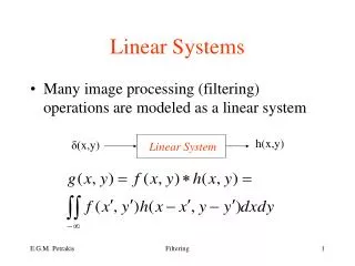
Linear Systems. Many image processing (filtering) operations are modeled as a linear system. h(x,y). δ( x,y). Linear System. δ( x,y). I. t. 0. Impulse Response. System’s output to an impulse δ (x,y). δ( x-x 0 ,y-y 0 ). h(x-x 0 ,y-y 0 ). Space Inv. Syst. af 1 (x,y)+bf 2 (x,y).

Linear Systems
E N D
Presentation Transcript
Linear Systems • Many image processing (filtering) operations are modeled as a linear system h(x,y) δ(x,y) Linear System Filtering
δ(x,y) I t 0 Impulse Response • System’s output to an impulse δ(x,y) Filtering
δ(x-x0,y-y0) h(x-x0,y-y0) Space Inv. Syst. af1(x,y)+bf2(x,y) ah1(x,y)+bh2(x,y) LSI System Space Invariance • g(x,y) remains the same irrespective of the position of the input pulse • Linear Space Invariance (LSI) Filtering
Discrete Convolution • The filtered image is described by a discrete convolution • The filter is described by a n x m discrete convolution mask Filtering
Computing Convolution • Invert the mask g(i,j) by 180o • not necessary for symmetric masks • Put the mask over each pixel of f(i,j) • For each (i,j) on image h(i,j)=Ap1+Bp2+Cp3+Dp4+Ep5+Fp6+Gp7+Hp8+Ip9 Filtering
Image Filtering • Images are often corrupted by random variations in intensity, illumination, or have poor contrast and can’t be used directly • Filtering: transform pixel intensity values to reveal certain image characteristics • Enhancement: improves contrast • Smoothing: remove noises • Template matching:detects known patterns Filtering
Template Matching • Locate the template in the image Filtering
Computing Template Matching • Match template with image at every pixel • distance 0 : the template matches the image at the current location • t(x,y): template • M,N size of the template Filtering
background constant correlation: convolution of f(x,y) with t(-x,-y) Filtering
true best match image correlation template noise false match Filtering
Observations • If the size of f(x,y) is n x n and the size of the template is m x m the result is accumulated in a (n-m-1) x (n+m-1) matrix • Best match: maximum value in the correlation matrix but, • false matches due to noise Filtering
Disadvantages of Correlation • Sensitive to noise • Sensitive to variations in orientation and scale • Sensitive to non-uniform illumination • Normalized Correlation(1:image, 2:template): • E : expected value Filtering
Histogram Modification • Images with poor contrast usually contain unevenly distributed gray values • Histogram Equalization is a method for stretching the contrast by uniformly distributing the gray values • enhances the quality of an image • useful when the image is intended for viewing • not always useful for image processing Filtering
Example • The original image has very poor contrast • the gray values are in a very small range • The histogram equalized image has better contrast Filtering
Histogram Equalization Methods • Background Subtraction: subtract the “background” if it hides useful information • f’(x,y) = f(x,y) – fb(x,y) • Static & Dynamic histogram equalization methods • Histogram scaling (static) • Statistical scaling (dynamic) Filtering
Static Histogram Scaling • Scale uniformly entire histogram range: • [z1,zk]: available range of gray values: • [a,b]: range of intensity values in image: • scale [a,b] to cover the entire range [z1,zk] • for each z in [a,b] compute • the resulting histogram may have gaps Filtering
Statistical Histogram Scaling • Fills all histogram bins continuously • pi: number of pixels at level ziinput histogram • qi : number of pixels at level zioutput histogram • k1= k2=… : desired number of pixels in histogram bin • Algorithm: • Scan the input histogram from left to right to find k1: • all pixels with values z1,z2,…,zk-1 become z1 Filtering
Algorithm (conted) • Scan the input histogram from k1 and to the right to find k2: • all pixels zk1,zk1+1,…,zk2 become z2 • Continue until the input histogram is exhausted • might also leave gaps in the histogram Filtering
Noise • Images are corrupted by random variations in intensity values called noise due to non-perfect camera acquisition or environmental conditions. • Assumptions: • Additive noise: a random value is added at each pixel • White noise: The value at a point is independent on the value at any other point. Filtering
Common Types of Noise • Salt and pepper noise: random occurrences of both black and white intensity values • Impulse noise: random occurrences of white intensity values • Gaussian noise: impulse noise but its intensity values are drawn from a Gaussian distribution • noise intensity value: • k: random value in [a,b] • σ : width of Gaussian • models sensor noise (due to camera electronics) Filtering
Examples of Noisy Images • Original image • Original image • Salt and pepper noise • Impulse noise • Gaussian noise Filtering
Noise Filtering • Basic Idea: replace each pixel intensity value with an new value taken over a neighborhood of fixed size • Mean filter • Median filter • The size of the filter controls degree of smoothing • large filter large neighborhood intensive smoothing Filtering
Mean Filter • Take the average of intensity values in a m x n region of each pixel (usually m = n) • take the average as the new pixel value • the normalization factor mn preserves the range of values of the original image Filtering
Mean Filtering as Convolution • Compute the convolution of the original image with • simple filter, the same for all types of noise • disadvantage: blurs image, detail is lost Filtering
Size of Filter • The size of the filter controls the amount of filtering (and blurring). • 5 x 5, 7 x 7 etc. • different weights might also be used • normalize by sum of weights in filter Filtering
Examples of Smoothing • From left to right: results of 3 x 3, 5 x 5 and 7 x 7 mean filters Filtering
Median Filter • Replace each pixel value with the median of the gray values in the region of the pixel: • take a 3 x 3 (or 5 x 5 etc.) region centered around pixel (i,j) • sort the intensity values of the pixels in the region into ascending order • select the middle value as the new value of pixel (i,j) Filtering
Computation of Median Values • Very effective in removing salt and pepper or impulsive noise while preserving image detail • Disadvantages: computational complexity, non linear filter Filtering
Examples of Median Filtering • From left to right: the results of a 3 x 3, 5 x 5 and 7 x 7 median filter Filtering
Gaussian Filter • Filtering with a m x m mask • the weights are computed according to a Gaussian function: • σis user defined Example: m = n = 7 σ2 = 2 Filtering
Properties of Gaussian Filtering • Gaussian smoothing is very effective for removing Gaussian noise • The weights give higher significance to pixels near the edge (reduces edge blurring) • They are linear low pass filters • Computationally efficient (large filters are implemented using small 1D filters) • Rotationally symmetric (perform the same in all directions) • The degree of smoothing is controlled by σ (larger σfor more intensive smoothing) Filtering
Gaussian Mask • A 3-D plot of a 7 x & Gaussian mask: filter symmetric and isotropic Filtering
Gaussian Smoothing • The results of smoothing an image corrupted with Gaussian noise with a 7 x 7 Gaussian mask Filtering
Computational Efficiency • Filtering twice with g(x) is equivalent to filtering with a larger filter with • Assumptions Filtering
Observations • Filter an image with a large Gaussian • equivalently, filter the image twice with a Gaussian with small σ • filtering twice with a m x n Gaussian is equivalent to filtering with a (n + m - 1) x (n + m - 1) filter • this implies a significant reduction in computations Filtering
Gaussian Separability Filtering
1-D Gaussian horizontally 1-D Gaussian vertically • The order of convolutions can be reversed Filtering
An example of the separability of Gaussian convolution • left: convolution with vertical mask • right: convolution with horizontal mask Filtering
Gaussian Separability • Filtering with a 2D Gaussian can be implemented using two 1D Gaussian horizontal filters as follows: • first filter with an 1D Gaussian • take the transpose of the result • convolve again with the same filter • transpose the result • Filtering with two 1D Gausians is faster !! Filtering
Noisy image • Convolution with 1D horizontal mask • Transposition • Convolution with same 1D mask • Transposition smoothed image Filtering