Download
1 / 47
470 likes | 625 Views
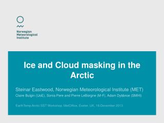
Ice and Cloud masking in the Arctic. Steinar Eastwood, Norwegian Meteorological Institute (MET) Claire Bulgin (UoE), Sonia Pere and Pierre LeBorgne (M-F), Adam Dybbroe (SMHI). Outline. Existing cloud/ice classification algorithms Probabilistic approach and PDFs Collection of training data

E N D
Ice and Cloud masking in the Arctic Steinar Eastwood, Norwegian Meteorological Institute (MET) Claire Bulgin (UoE), Sonia Pere and Pierre LeBorgne (M-F), Adam Dybbroe (SMHI)
Outline Existing cloud/ice classification algorithms Probabilistic approach and PDFs Collection of training data Adapting existing PDFs to new sensors Twilight conditions AATSR, South-east coast of Greenland
Conventional classification algorithms General cloud/ice/water classification algorithms often wants to provide an unbiased cloud classification Hence some clouds are undetected SST retrieval would like a more certain/conservative classification Need additional cloud and ice masking step after applying conventional cloud mask Especially for sea ice since this is often less accurately handled by general cloud classification algorithms Also need particulare focus on twilight conditions since more frequent at high latitudes
Probabilistic approach Method is based on probability distribution functions (PDF) for channel features, often combined using Bayes theorem Gives the probability of the satellite data being cloudy, water and ice given the observations Provides flexible method, the additional masking can be tuned on the probabilities Need classified data to define/train PDFs
Classification example 2009-04-14 AATSR
Ways of collection training data Good/representative PDFs depend on good training data Three methods: Manual classification (eg. MET Norway) Automatic classification with ground truth, such as synop, cloud satellite missions and sea ice products (eg. SMHI) Using existing cloud mask as «truth», such as PPS, Maia, SADIS, CLAVR-X (eg. Chris, Owen, Claire)
Automatic collection of training data with Calipso cloud lidar on Caliop Looking at Calipso cloud lidar data collocated with VIIRS data and ice concentration for collection of training data (cooperation with SMHI) Using VIIRS orbits which Caliop crosses close in time Use Calipso to define/classify cloudy and cloud free areas, even over ice Can then define the PDFs for cloud, ice and water Still need to separate ice from water, as Calipso only sees clouds
Using PPS as «truth» Have used one year of collocated VIIRS data and PPS cloud mask Use PPS to define areas with clouds, clear sea, clear ice, clear land and clear snow At night, PPS only classify cloud and clear So apply simple test to split ice and sea: ice if clear & T11 < 270 water if clear & T11 > 275
Using PPS as «truth» Build count matrix (multi-dim histogram) by looping through all scenes Calculate the channel feature(s) we want (eg. 0.9/0.6, std(0.6)) Summarize how many pixels in each class in defined intervals in these feature(s) Save this matrix in NetCDF file Have made Python tool to visulize these histograms in 3D, 2D and 1D Can also compare matrixes from two different satellites
Training data: Calipso vs PPS Comparing 2D histograms of training data Both are one year of locally received data at SMHI, Sweden Calipso in red PPS in blue r0.9um/r0.6um vs sunz
3D view of nighttime matrix Water Sea Ice Cloud
How to define the PDFs Parameterize histograms as analytic probability functions Typically use Gaussian normal distribution • Define look-up tables from training data, 1D or multi-dimensional • Needs lots of data for multi-dim
Defining PDFs for new instruments How to adapt existing coefficients / method to new instruments Options: Repeat manual classification training – expensive... Compare overlapping orbits from new and old instrument Simulate difference between existing and new instruments Some examples...
New PDFs for NPP VIIRS The OSI SAF method had coefficients for AVHRRs on NOAA17,18,19 and METOP-A We needed to updated the OSI SAF method to work on VIIRS data (during day) Had no time to do an extended training of method by manual classification Wanted to adjust the existing N19 AVHRR coefficients to VIIRS Comparing N19 and NPP orbits close in time (+/- 0.5 hour)
NPP VIIRS r0.9um/r0.6um N19 AVHRR 02.06.2012
NPP VIIRS PDFs Use the limited set of collocated VIIRS + AVHRR data to find average shift between PDFs for this limited set Apply this average shift to define overall VIIRS PDFs: PDFVIIRS = PDFAVHRR - shift(AVHRR-VIIRS) VIIRS chain at CMS/MF run with these new coefficients and work fine
Simulating ref Chris and Owen...
Twilight Some of the features/channel combinations we use deviates from the normal day light behaviour when approaching twilight
AVHRR 0.8um/0.6um , sea norm + PDF Sunz < 80: PDFmean = MB PDFstd = SB Sunz 80-90: PDFmean = MA*SOZ + MB PDFstd = SA*SOZ + SB
Simulating twilight Have just started to simulate visible channels using libradtran Example with r0.9/r0.6 for water and snow
Arctic Challenges How to train PDFs to cope with difficult conditions Twilight Ice vs clouds and wet ice vs cold water during night How thick is the ice before we can distinguish it from water Find good validation data for comparing algorithms under these challenging conditions How does different performance of cloud/ice mask at day / twilight / night influence SST accuracies? Should we try to see how SST accuracies varies with cloud masking skill from PDFs?
From Metop02 to Metop01 The AVHRR on Metop02 and Metop01 should be very similar Will building channel count matrixes for both satellites with 6 months of Arctic data Classification is based on Maia cloud mask and OSI SAF sea ice concentration information
From Metop02 to Metop01 r0.9um/r0.6um June 2013 1 – Metop01 2 – Metop02
Additional 0.6um test Some ice were still classified as open water, espesially melting ice with low 0.9um/0.6um values Sonia and Pierre suggested an additional test using 0.6um to mask undetected ice Defined static threshold test Could introduce PDF
Improving cloud and ice masking algorithm at high latitudes during ESA CCI on SST
Cloud and ice masking in ESA CCI SST Training of method for cloud and ice masking has been based on manual classification This has been done by visual inspection and classification of areas within satellite scenes ICE WATER CLOUD
Cloud and ice masking in ESA CCI SST Have collected scenes close to sea ice border from different satellites, months, day/night/twilight Also use this data set for validation This data set will be published for all interested to access Using GAC data 1/4: ice, 2: clouds, 3: water
Update of algorithm Want to improve masking during twilight and night Have looked at dependency on sun zenith angle for the PDFs Using existing cloud mask (CLAVR-X) from the HL MMD to study cloud signatures for all seasons, in areas close to the ice edge
VIIRS 0.8um/0.6um , sea norm + PDF Sunz < 80: PDFmean = MB PDFstd = SB Sunz 80-90: PDFmean = MA*SOZ + MB PDFstd = SA*SOZ + SB
VIIRS 0.8um/0.6um , sea ice , normalized Fewer data...
Daytime bt3.7-bt11 PDFmean = MA*SOZ + MB PDFstd = SA*SOZ + SB
Nighttime VIIRS, distance to WTP Distance to water tiepoint Line defining water tiepoints
Day time algorithms uses: r0.9/r0.6 and r1.6/r0.6 or r0.9/r0.6 and bt3.7-bt11 Must add r0.6... Night time algorithm uses: dist(bt3.7-bt11, bt11-bt12) LSD(bt3.7-bt11) , log-normal distribution