Download
1 / 1
10 likes | 160 Views
Polar Science Center. Lindsay@apl.washington.edu. Air, Ocean, Earth, and Ice on the Rock CMOS-CGU-AMS Congress 2007 28 May to 1 June, St John’s Newfoundland Poster 1604, Operational Oceanography. Seasonal Predictions of Ice Extent in the Arctic Ocean

E N D
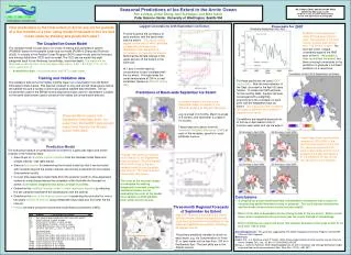
Polar Science Center Lindsay@apl.washington.edu Air, Ocean, Earth, and Ice on the Rock CMOS-CGU-AMS Congress 2007 28 May to 1 June, St John’s Newfoundland Poster 1604, Operational Oceanography Seasonal Predictions of Ice Extent in the Arctic Ocean Ron Lindsay, Jinlun Zhang, Axel Schweiger, and Mike Steele Polar Science Center, University of Washington, Seattle WA Lagged Correlations with September Ice Extent Forecasts for 2007 How predictable is the total extent of Arctic sea ice for periods of a few months to a year using model hindcasts of the ice and ocean state for training and prediction data? The Coupled Ice-Ocean Model The hindcast model is a pan-arctic ice–ocean modeling and assimilation system (PIOMAS) based on the parallel ocean and ice model (POIM) of Zhang and Rothrock (2003). It consists of the Parallel Ocean Program (POP) ocean model and the thickness and entropy distribution (TED) sea ice model. The TED sea ice model has eight categories each for ice thickness, ice enthalpy, and snow depth; The maximum ice thickness in each bin is 0.10 m (the open water class), 0.66, 1.93, 4.20, 7.74, 12.74, 19.31, and 27.51 m. • Assimilation data: ice concentration and SST in open water Training and Validation data The validation data set is the Hadley monthly mean ice concentration from the British Atmospheric Data Centre. This data set is based on ship and aircraft observations before the satellite era and a variety of active and passive satellite data thereafter. The ice concentration used in the ERA40 forcing data set and also used for assimilation is based on the same data stream used to construct the Hadley Ice concentration data set. Prediction of the September mean total ice extent for this year. The predictor is the area fraction of water and ice less than 1.93 m thick in April. The error bar is the 1-sigma uncertainty equal to the RMS error of the fit. We predict a near record low ice extent, but there is enough uncertainty in the prediction to preclude a confident prediction of a record low. First we examine the correlation of each predictor with the basin-wide total ice extent. This figure showslagged correlations of each candidate variable with the basin-wide September mean ice extent: a) Correlations, b) Squared correlations Note that the climate indexes in the upper plot are off the bottom in the lower plot. At 1 and 2 months lead ice concentration is best correlated with the ice extent. At longer leads the ocean temperature at 234 m is best correlated. Based on ERA-40 forcing data. For these predictions we used NCEP forcing data. Now the best estimator of the Sept. ice extent is the April G2 area fraction. To obtain the CWT estimate for the monthly fields, the April G2 area is averaged with a weighting proportional to the correlation of each point with the September total ice extent. This map shows the correlation field used to generate the correlation weighted time series. Correlations are negative because lots of thin ice in April leads to lots of summer open water and low ice extent. Predictions of Basin-wide September Ice Extent Correlation maps of the pan-arctic September mean ice extent for four different variables at different lead times. July is a lead of 2 months, March is a lead of 6 months, and November is a lead of 10 months These maps are used to form the correlation-weighted time series (CWT) of each of the variables, specific for each particular lead time. Observed March (upper) and September (lower)pan-arctic ice extent from the HadSST data set with linear trend lines for the 48-year period 1958–2005. These maps show the anomalies (relative to 1970-2006) of the April G2 area fraction for the last four years and show that the area of open water and thin ice is greatest in the last year, leading to the prediction of near record low ice extent for this summer. • Prediction Model • The forecast procedure for predicting the ice extent for a particular region and month consists of the following steps: • Select a set of candidate forecast variables from the hindcast model fields and climate indexes (see table below). • Select a time interval for determining the forecast model (so that it can be tested with forecasts beyond the chosen interval) and choose a lead time for the forecast (the predictor month). • Convert time-dependent model fields (from the predictor month) to time-dependent scalars in a way that preserves the correlation of the field with the forecast ice extent. (Correlation weighted time series, Drobot et al 2006). • Determine the statistical forecast model, alinear regression equation by selecting the two variables that best fit the observations over the interval. • Determine the error of the forecast expression in predicting the ice extent for one or two years after the fit interval, using independent input data also from after the the interval. • Predict ice extent using the most recent model fields (converted to CWTs). Candidate Variables Forecast skill scores for the pan-arctic forecast of the September mean ice extent. The line marked Fit is the R2 value of the two-variable model fit over the entire time interval. The other lines are the forecast skill scores. The error of the forecast model is evaluated by making prognostic forecasts using the statistical model, not on evaluating the error of the model for a sample of withheld data from within the fit interval. • Conclusions: • A coupled ice-ocean model provides considerable information that is useful in constructing skillful forecasts a year in advance. The ice thickness distribution and the ocean temperatures are particularly helpful. • Much of the skill is dependent on the strong trends in the ice extent. Skill is much lower when compared to the previous year ice extent instead of climatology. • Near record low ice extent will occur this summer because of the large extent of ice less than 1.93 m thick. • Acknowledgements: This work was supported by The NASA Cryospheric Sciences Program and the NSF Office of Polar Programs. • References • Drobot, S.D., J.A. Maslanik, and C.F. Fowler, 2006: A long-range forecast of Arctic summer sea-ice minimum extent. Geophy. Res. Lett., 33, doi:10.1029/2006GL026216. • Zhang, J., and D.A. Rothrock, 2003: Modeling global sea ice with a thickness and enthalpy distribution model in generalized curvilinear coordinates, Mon. Wea. Rev., 131(5), 681–697. • Three-month Regional Forecasts of September Ice Extent • Map of R2 values of the model fit (thin bars) and the climate-relative forecast skill scores (thick bars) of three-month predictions for the observed September ice extent in individual 45-degree sectors. • The primary predictive variable is shown for each sector, e.g. Ice Concentration for Fram St, or open water and ice less than 1.93 m in the Barents Sea. The best skills are in the Atlantic sectors. Predictor variable R2 Skill vs climatology