Download
1 / 38
380 likes | 549 Views
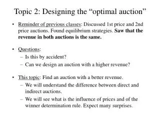
Topic 2: Designing the “optimal auction”. Reminder of previous classes : Discussed 1st price and 2nd price auctions. Found equilibrium strategies. Saw that the revenue in both auctions is the same. Questions : Is this by accident? Can we design an auction with a higher revenue?

E N D
Topic 2: Designing the “optimal auction” • Reminder of previous classes: Discussed 1st price and 2nd price auctions. Found equilibrium strategies. Saw that the revenue in both auctions is the same. • Questions: • Is this by accident? • Can we design an auction with a higher revenue? • This topic: Find an auction with a better revenue. • We will understand the difference between direct and indirect auctions. • We will see what is the influence of prices and of the winner determination rule. Expect many surprises.
The Revelation Principle • Problem: there are infinitely many possible auction formats, so it is hard to go over all of them… • Reminder: In a direct-revelation auction, the strategy space of a player is simply to report her type (value). THM: Given any auction format with equilibrium strategies s(), there exists a direct-revelation auction for which truthfulness is an equilibrium, with the same outcome, and the same prices. • Remark: This holds for any type of equilibrium (dominant strategies, Bayesian-Nash,...) • The implication: we need only search for a direct-revelation auction.
Proof (sketch) New Auction • A proxy mimics the equilibrium strategy: if others are truthful, player i would like to play si(vi), so she needs to declare vi. • Examples: • In the 1st price auction, the proxy will convert vi to [(n-1)/n]vi • In the English auction, the proxy will take vi and will keep “raising the hand” until the price reaches vi. Input v Output s(v) Original Auction Original Output “Proxy”
How to set prices? • As we saw, there can be many ways to set prices. Which is best? • Surprisingly, prices also don’t matter!! THM (The Revenue Equivalence Theorem):Suppose vi is drawn independently from some Fi(x), which is continuous and strictly increasing on some interval [a,b].Take any two auctions such that, in both auctions: - The expected utility of a player with value a is the same. - The probability of a player that declares v to win is the same (assuming players play the equilibrium strategies).Then these two auctions raise the same expected revenue (in equilibrium) . • The 1st and 2nd price auctions satisfy all conditions (why??), so our analysis is an example to this general theorem.
How to set prices? • For simplicity we will assume that a=0 and that the expected utility of a player with value 0 is 0. In this case the theorem is: THM (The Revenue Equivalence Theorem):Suppose vi is drawn independently from some Fi(x), which is continuous and strictly increasing on some interval [0,b].Take any two auctions such that, in both auctions, the probability of a player that declares v to win is the same (assuming players play the equilibrium strategies).Then these two auctions raise the same expected revenue (in equilibrium) .
Proof (1) • By the revelation principle, we need only check truthful auctions (that get values, and output a winner and a price). Denote by: • Oi(v) the probability (over v-i) that i wins when declaring v. • Pi(v) the expected payment of I when she declares v. • ui(v) = v·Oi(v) – Pi(v) = i’s expected profit when declaring v.
Proof (1) • By the revelation principle, we need only check truthful auctions (that get values, and output a winner and a price). Denote by: • Oi(v) the probability (over v-i) that i wins when declaring v. • Pi(v) the expected payment of I when she declares v. • ui(v) = v·Oi(v) – Pi(v) = i’s expected profit when declaring v. • Truthfulness in equilibrium is equivalent to the condition that, for every v,v’ :ui(v) = v·Oi(v) – E[i’s price when declaring v] >v·Oi(v’) – E[i’s price when declaring v’] = ui(v’)+(v-v’) Oi(v’)
Proof (1) • By the revelation principle, we need only check truthful auctions (that get values, and output a winner and a price). Denote by: • Oi(v) the probability (over v-i) that i wins when declaring v. • Pi(v) the expected payment of I when she declares v. • ui(v) = v·Oi(v) – Pi(v) = i’s expected profit when declaring v. • Truthfulness in equilibrium is equivalent to the condition that, for every v,v’ :ui(v) = v·Oi(v) – E[i’s price when declaring v] >v·Oi(v’) – E[i’s price when declaring v’] = ui(v’)+(v-v’) Oi(v’) • By exactly the same argument:ui(v’) > ui(v)+ (v’-v) Oi(v)
Proof (2) • Denote dv = v-v’. Rewriting what we have:ui(v) > ui(v’)+dv Oi(v’) ; ui(v’) > ui(v)- dv Oi(v)
Proof (2) • Denote dv = v-v’. Rewriting what we have:ui(v) > ui(v’)+dv Oi(v’) ; ui(v’) > ui(v)- dv Oi(v) dv Oi(v) > ui(v) - ui(v’) > dv Oi(v’)
Proof (2) • Denote dv = v-v’. Rewriting what we have:ui(v) > ui(v’)+dv Oi(v’) ; ui(v’) > ui(v)- dv Oi(v) dv Oi(v) > ui(v) - ui(v’) > dv Oi(v’)Oi(v’+dv) >[ui(v’+dv) - ui(v’)]/dv > Oi(v’)
Proof (2) • Denote dv = v-v’. Rewriting what we have:ui(v) > ui(v’)+dv Oi(v’) ; ui(v’) > ui(v)- dv Oi(v) dv Oi(v) > ui(v) - ui(v’) > dv Oi(v’)Oi(v’+dv) >[ui(v’+dv) - ui(v’)]/dv > Oi(v’)Letting dv approach zero => dui/dv = Oi(v)
Proof (2) • Denote dv = v-v’. Rewriting what we have:ui(v) > ui(v’)+dv Oi(v’) ; ui(v’) > ui(v)- dv Oi(v) dv Oi(v) > ui(v) - ui(v’) > dv Oi(v’)Oi(v’+dv) >[ui(v’+dv) - ui(v’)]/dv > Oi(v’)Letting dv approach zero => dui/dv = Oi(v)=> ui(v) = 0v Oi(x)dx
Proof (2) • Denote dv = v-v’. Rewriting what we have:ui(v) > ui(v’)+dv Oi(v’) ; ui(v’) > ui(v)- dv Oi(v) dv Oi(v) > ui(v) - ui(v’) > dv Oi(v’)Oi(v’+dv) >[ui(v’+dv) - ui(v’)]/dv > Oi(v’)Letting dv approach zero => dui/dv = Oi(v)=> ui(v) = 0v Oi(x)dx • We get Pi(v) = v·Oi(v) - ui(v) =v·Oi(v) - 0v Oi(x)dxThus Pi(v) depends only on the outcome function Oi(·).Since these are identical for both mechanisms, so is the revenue.
Picture Oi(vi) Pi(v) = v·Oi(v) - 0v Oi(x)dx 1 Oi(vi) 0 vi vi b Pi(vi)
Proof (3) • Since E[i’s price] = ab f(v) Pi(v) dv ,it follows that this too is identical to both mechanisms. • Since E[Total revenue] = iE[i’s price], the total expected revenue is also identical.
Conclusion: To design a revenue-maximizing auction, the only question is who will be the winner (in equilibrium). (And since the player with highest value wins both in the 1st and 2nd price auctions, their revenues are equal)
A characterization of truthfulness • We saw that, to maximize revenue, we only need to search for allocation rules Oi(·). But what allocation rules can be implemented? I.e. for which allocation rules we can add prices that will make the auction truthful? THM: An auction is truthful if and only if(i) Oi(·) is non-decreasing.(ii) Pi(v) = v·Oi(v) – av Oi(x)dx • Note that (i) and (ii) were obtained as part of the proof of the revenue equivalence theorem. • The necessity part (truthfulness implies (i)+(ii)) was shown as part of the proof of the Revenue Equivalence theorem.
Proof of sufficiency • Since ui(v) = v·Oi(v) – Pi(v) we have ui(v) =av Oi(x)dx • Recall that truthfulness is equivalent to the conditionui(v’) > ui(v)+ (v’-v) Oi(v)
Proof of sufficiency • Since ui(v) = v·Oi(v) – Pi(v) we have ui(v) =av Oi(x)dx • Recall that truthfulness is equivalent to the conditionui(v’) > ui(v)+ (v’-v) Oi(v) • So fix any v’,v. • If v’ > v then:ui(v’) - ui(v)= vv’Oi(x)dx ( by (ii) )>vv’ Oi(v)dx ( by (i) ) = (v’ – v) Oi(v)
Proof of sufficiency • Since ui(v) = v·Oi(v) – Pi(v) we have ui(v) =av Oi(x)dx • Recall that truthfulness is equivalent to the conditionui(v’) > ui(v)+ (v’-v) Oi(v) • So fix any v’,v. • If v’ > v then:ui(v’) - ui(v)= vv’Oi(x)dx ( by (ii) )>vv’ Oi(v)dx ( by (i) ) = (v’ – v) Oi(v) • If v’ < v then:ui(v’) - ui(v)= -v’vOi(x)dx ( by (ii) )> -v’v Oi(v)dx ( by (i) ) = -(v – v’) Oi(v)
Prices and virtual valuation • Let (v) = v - (1-F(v))/f(v). Call it the “virtual value” function. Claim: Evi[Pi(vi)] = Evi[(vi)·Oi(vi)] • Interpretation: The best revenue that the auctioneer can hope to extract from a player is vi ·Oi(vi). The claim tells us that (in expectation) it can extract less, at most (vi)·Oi(vi).
Prices and virtual valuation • Let (v) = v - (1-F(v))/f(v). Call it the “virtual value” function. Claim: Evi[Pi(vi)] = Evi[(vi)·Oi(vi)] Proof: Recall that Pi(v) = v·Oi(v) – av Oi(x)dx. Therefore: Evi[Pi(vi)] = ab Pi(v)f(v)dv = =ab v·Oi(v)·f(v)dv - ab f(v) av Oi(x)dx dv = ab v·Oi(v)·f(v)dv - ab Oi(v)(1-F(v)) dv = ab f(v)·Oi(v)·[v - (1-F(v))/f(v)]dv = ab f(v)·Oi(v)· (v) dv = Evi[(vi)·Oi(vi)] Explanation to this in the next slide
Explanation delayed from previous slide Let G(v) = av Oi(x)dx. Define F(v)·G(v) = W(v). Then: F(b)·G(b) = W(b) =ab W’(v)dv = = ab F’(v)·G(v)dv + ab F(v)·G’(v)dv = = ab f(v)·G(v)dv + ab F(v)·Oi(v) dv = = ab f(v)· av Oi(x)dx dv + ab F(v)·Oi(v) dv => ab f(v)· av Oi(x)dx dv = F(b)·G(b) - ab F(v)·Oi(v) dv = = 1· ab Oi(v)dv - ab F(v)·Oi(v) dv = ab Oi(v)(1-F(v)) dv
What is the revenue of the auction? • Define: • Oi(v1…vn) the probability that player i wins when all the declarations are v1…vn. Note that Oi(vi) = Ev-i[Oi(vi,v-i) ]. • Pi(v1…vn) the probability that player i wins when all the declarations are v1…vn. Note that Pi(vi) = Ev-i[Pi(vi,v-i) ].
What is the revenue of the auction? • Define: • Oi(v1…vn) the probability that player i wins when all the declarations are v1…vn. Note that Oi(vi) = Ev-i[Oi(vi,v-i) ]. • Pi(v1…vn) the probability that player i wins when all the declarations are v1…vn. Note that Pi(vi) = Ev-i[Pi(vi,v-i) ]. • Conclusion: the expected revenue of the auction is: Ev1…vn [iPi(v1…vn)] =iEv1…vn [Pi(v1…vn)]=iEvi[Ev-i[Pi(vi,v-i) ]] = iEvi[Pi(vi)] = iEvi[(vi)·Oi(vi)] = iEvi[(vi)·Ev-i[Oi(vi,v-i) ]] = iEv1…vn [(vi)·Oi(v1…vn)] = Ev1…vn [i(vi)·Oi(v1…vn)]
What is the optimal auction? Conclusion: the expected revenue of the any auction must be Ev1…vn [i(vi)·Oi(v1…vn)] • How to maximize this? Choose the winner to be the player with the maximal virtual valuation, unless all virtual valuations are negative, and then no one wins. • Is this truthful? If and only if the virtual valuation function is monotone.
A more convenient formulation • Since virtual valuations are non-decreasing, this means that the player with the highest value has the highest marginal valuation. • One exception: if (v) < 0 then no one wins. This happens for every v < v* where v* solves v = (1-F(v))/f(v). • By the revenue equivalence theorem, this means that a 2nd price auction with a reservation price v* is a revenue maximizing auction.
Remark for asymmetric bidders • If player values are drawn from different distributions, all the analysis we’ve done still holds. • However, the marginal valuation functions will be different between players, and so we cannot use the convenient format just described. • This also means that it is not necessarily the case that the player with the highest value will win. This depends on the shape of the virtual valuation functions.
Some problems with assumptions of the revenue equivalence theorem • Budget constraints: bidders may not be able to pay their value. • Asymmetries in probability distributions - this by itself does not violate the statement but it may violate the outcome equivalence (1st price may not give the item to the bidder with the highest value). • Bidders may not be risk-neutral. • Interdependent valuations: values of players are related in some way.
Risk Neutrality in the Analysis DFN: The strategies s1,…, snare in Bayesian-Nash equilibrium if for any i, vi, ai : Ev-i[ui(si(vi),s-i(v-i)] > Ev-i[ui(ai,s-i(v-i)] But for the analysis of the 1st price auction, and for the proof of the revenue equivalence theorem, we actually assume that the player chooses a bid b to maximize his expected profit: Ev-i[value- price | i bids b] • Thus, a crucial assumption is:utility from expectation = expected profit • This is termed risk-neutral players. • Thus, it is an assumption for the revenue equivalence theorem. • But sometimes this is not true. For example, we might care about the variance (smaller variance might be better).
Risk aversion in 1st and 2nd price auctions • In a 2nd price auction, the dominant strategy is to bid truthfully, so risk-aversion does not change anything. • There is no expectation in the considerations of a player -- dominant strategy maximizes the player’s utility, no matter what the others are doing. • In a 1st price auction, the equilibrium we calculated is a Bayesian-Nash equilibrium, so risk-aversion might change the picture.
Sensitivity to risk • This is usually modeled by a von-Neumann – Morgenstern utility: • We have a utility function ui: R -> R. The utility of a given profit x ( = value minus price) is ui(x). • The utility of a lottery p is the expected utility:ui(p)= xp(x)ui(x) • Thus players maximize the expectation of utility of profit. This might be different than the expectation of profit.
Example 1 – risk neutral players u(x) u(x)=x The lottery: with probability 0.5 a profit of 4, with probability 0.5 a profit of 1 u(0.5 · 4 + 0.5 · 1) = u(2.5)=2.5 0.5 u(4) + 0.5 u (1) = 0.5 · 4 + 0.5 · 1 = 2.5 Conclusion: the lottery and receiving the mean for sure are equivalent for the player. u(4)=4 u(1)=1 x 1 4
Example 2 – risk averse players u(x) The lottery: with probability 0.5 a profit of 4, with probability 0.5 a profit of 1 u(0.5 · 4 + 0.5 · 1) = u(2.5)1.58 0.5 u(4) + 0.5 u (1) = 0.5 · 2 + 0.5 · 1 = 1.5 Conclusion: the lottery is worse than receiving the mean for sure. u(x)=x u(4)=2 u(1)=1 x 1 4
Risk-aversion in first-price auctions THM: Suppose that players are risk-averse, with the same utility function u, and that values are drawn independently from the same distribution F (with bounded support). Then the expected revenue of the symmetric equilibrium of a first-price auction is not smaller than the expected revenue of the second-price auction. Remarks:(1) There is only one unique symmetric equilibrium.(2) No asymmetric equilibria exist (unless the support is not bounded).[We will not prove anything]
The picture Revenue of 1st price with risk-aversion > Revenue of 1st price with risk-neutrality = Revenue of 2nd price with risk-neutrality = Revenue of 2nd price with risk-aversion There are examples where the revenue is strictly higher in a 1st price auction, and examples where the revenue is equivalent.