A Look at the Interior of Mars

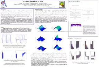
1. A Look at the Interior of Mars A. Khan(1), K. Mosegaard(2), Philippe Lognonné(1) and M. Wieczorek(1) (1) Département de Géophysique Spatiale et Planétaire, Institut de Physique du Globe de Paris (2) Niels Bohr Institute, University of Copenhagen, Denmark khan@ipgp.jussieu.fr Bayesian Hypothesis Testing Method of Analysis Introduction The existence of a martian core has been widely accepted for some time and even more so now given its ability to explain in a natural way the presence of the strong, spatially variable magnetic fields found by the MGS spacecraft. An ancient internal dynamo is assumed to have been present, magnetising crustal material as it cooled through the Curie temperature. Other supporting evidence comes from the SNC meteorites, in the form of their siderophile element depletion. These are thought to have been removed during core formation. The present analysis is concerned with a rigorous inversion of a set of currently available geophysical data that provides information on the deep interior structure of Mars. The data used in the inversion are, mean moment of inertia (I/MR2), mean density (), second degree tidal Love number (k2) and tidal dissipation factor (Q). Their values are, in this order, 0.36360.0017, 39330.4 kg/m3, 0.1450.017, 9211 (referenced to a mean radius of 3389.5 km. Forward problem - Our model of Mars is assumed spherically symmetric and divided into 7 shells of variable size. Each one of these shells is physically described by a number of parameters, which are, bulk and shear modulus, density, local dissipation factor and radial extent of the layer (no correlation among the elastic parameters is assumed). From this model I, , Q and k2 can be calculated. Inverse problem - The inversion is conducted using a non-linear inverse Monte Carlo sampling technique, involving the use of probability density functions to represent every single state of information. The inverse problem is then formluated as a conjunction of states of information and the outcome represented by the posterior probability distribution contains all the information provided by data, prior information and any theoretical correlations that may exist between data and model parameters. The posterior results will be analysed according to a Bayesian scheme. Slide 1 We have used the Bayes factor to estimate which scenario, among the following two is the most likely for Mars, given prior information and data. we distinguish between two end-member models, one where Mars has entirely solid core and one where Mars has an entirely molten core. These are essentially our two hypotheses that we wish to distinguish between. The Figure on the left shows the likelihood function, which is a measure of how well data are fit, for these two runs (blue - solid core, red - liquid core). Using Eq. 13 above leads to a Bayes factor of 0.00004, thereby indicating that the fluid core model is the most probable outcome. Results Samples from the posterior distribution are in the figures, showing S-wave velocity, density and Q as a function of radius. We have also displayed 2D-marginals to highlight the correlation that exists among the parameters, notably density and radius. To be able to gain a better insight into the sensitivity of the individual data, we have also displayed prior information. Another example of prior and posterior models. Here we have displayed 2D posterior marginal distributions to investigate the correlation between two parameters, here S-wave velocity and radius. Results from the initial inversion Samples from the prior (left) and posterior probability (right) distributions. The figures show S-wave velocity, Q and density as a function of radius. The spread of the posterior samples is a measure of how well resolved the interior structure models are. This is most clearly seen in the case of the S-wave velocity and density models. Of prime interest in a study like this, is to get an idea of how sensitive data actually are to the individual parameters as a function of depth. It is our hope to be able to adress several questions concerning the structure of Mars, especially those regarding the state, size and density of the core. The Love number is known to be sensitive to the state of the core, but less to its density. With the series of figures above we investigate this question. The figures show from top to bottom results from an inversion of only prior information, all data and results from an inversion of only mass and moment of inertia. The column to the left shows the 2D marginal ppd’s of density vs. radius for the shell situated just below the core/mantle boundary, whereas the one to the right the same information, but here for the shell immediately above the core/mantle boundary. Comparison of these figures provides an indication of the sensitivity of the Love number to the deep interior structure of Mars, notably the density. Another example of prior and posterior models. Here we have displayed 2D posterior marginal distributions to investigate the correlation between two parameters, here S-wave velocity and radius. Prior and posterior density and S-wave velocity models for the two runs used in the estimation of the Bayes factor. The left column shows liquid core models, whereas the one on the right shows solid core models. A. Khan acknowledges the financial support provided through the European Community\s Human Potential Programme under contract RTN2-2001-00414, MAGE.