SCIENCE INSTRUMENTS
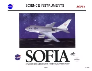
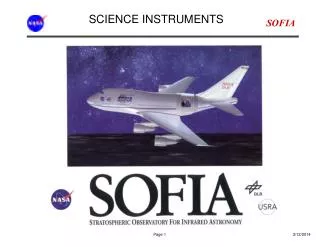
SCIENCE INSTRUMENTS. SOFIA’s Instrument Complement. As an airborne mission, SOFIA has a unique, wide instrument complement SOFIA covers the full IR range with imagers and low, moderate, and high resolution spectrographs

SCIENCE INSTRUMENTS
E N D
Presentation Transcript
SOFIA’s Instrument Complement • As an airborne mission, SOFIA has a unique, wide instrument complement • SOFIA covers the full IR range with imagers and low, moderate, and high resolution spectrographs • 4-5 instruments at Initial Operational Capability (IOC); 8-9 instruments at Full Operational Capability (FOC) • SOFIA can take full advantage of improvements in instrument technology • Both Facility and PI Instruments
SOFIA Science Missions Circumstellar Disks EXES, FORCAST Galactic Center FORCAST, SAFIRE, HAWC Powering of ULIRGs SAFIRE, FIFI-LS, HAWC Extragalactic Star Formation SAFIRE, FIFI-LS, HAWC Transits of Extrasolar Planets HIPO Planets (e.g., Gas Giants, Titan, Pluto/Charon) HIPO, SAFIRE Deuterated Hydrogen (HD) GREAT CII cooling of the ISM GREAT, SAFIRE, FIFI-LS, CASIMIR Evolution of Matter in the Early Universe HAWC, SAFIRE Active Galactic Nuclei HAWC, SAFIRE Spectroscopy of protostars CASIMIR, GREAT, SAFIRE ISM Chemistry CASIMIR, GREAT Infall/Outflow around YSOs CASIMIR, GREAT, FIFI-LS SNR Impact on Molecular Clouds CASIMIR, GREAT, FIFI-LS Planet Formation EXES Water vapor in molecular clouds EXES, CASIMIR, GREAT
Far-IR Lines as Science Tools Many fine-structure and molecular-transition lines serve as probes of the physical properties of the ISM of the Milky Way and other galaxies: • [OI], [SiII] lines probe the physical conditions of gas in PDRs. • [NIII], [SIII], and [OIII] line pairs are excellent probes of HII region densities. • [NII] lines trace the warm ionized medium. • [CII] line traces PDRs, atomic clouds, and warm ionized medium. • [NII]/[NIII], [SIII]/[OIII], [NeIII]/[OIV]/[NeV] ratios give the effective temperature of stellar or AGN UV radiation fields. • [SI], [SiI], [SiII] and [FeI] lines indicate the presence of dissociative J-shocks. • High-J CO rotational lines trace shocked gas found in warm dense gas of PDRs. • OH lines trace shocked gas in cool dense gas. • H2 rotational lines probe the mass of warm molecular clouds. • OH, CH, and NH3 together constrain molecular cloud chemistry. • [CI] traces star formation, atomic clouds.
SI Performance Descriptions Purpose: provide uniform description of SI capabilities, adequate to judge feasibility of investigations Target: potential General Investigators Scope: all SOFIA instruments Format: uniform representation of each SI Content: spectral resolution/wavelength bands, angular resolution, sensitivity, basic operating modes, particulars, caveats
SI Performance Description - Preparation Sensitivity units are Jy for broad band instruments and W/m2for lines. Some equivalent values (e.g., magnitudes, TA*) are provided. Sensitivity measures are MDCF (continuum) and MDLF (lines) with a criterion of 4 sigma in 15 minutes = 900 s. PowerPoint and PDF versions available.
Predicted Image Quality vs. Wavelength Expected behavior of SOFIA images from wind tunnel test results and telescope FEM. Later improvement in pointing stability Potential with IMC and active optics
Wavelength Dependence of PSF 0.3 mm 1.0 mm 1.5 mm 2.0 mm
Predicted Image Quality vs. Wavelength( l 0.5 µm to l 100 µm )
SOFIA SI Spectral Resolution (km/s) vs. Wavelength CLICK ON INSTRUMENT BOX TO GO TO 3-PAGE SUMMARY GREAT CASIMIR EXES Km/s FIFI-LS SAFIRE FLITECAM FORCAST HAWC HIPO Wavelength (µm)
105 104 103 EXES Spectral Resolution Wavelength range: 5 - 28 µm Three Resolving Powers: High: ~ 105 Medium: ~ 104 Low: ~3000 The resolving power plotted corresponds to the FWHM of the instrument line spread function for a monochromatic line from a point source. Wavelength changes require about 3 minutes. Resolution change requires about 3 minutes. High Velocity Resolution (km/s) Spectral Resolving Power l/Dl Medium Low Wavelength (µm) Free spectral range : High: 1500 km/sec (echelle mode) Medium: 1500 km/sec Low: 6000 km/sec
EXES Sensitivity MDLF is the “minimum detectable line flux”, 4s in 15 minutes (900s) on-source integration time. MDLF is plotted for an unresolved line from a point source, for each of the three resolution modes, Low, Medium and High. MDLF scales roughly as (S/N)/√ t where t = net integration time Minimum detectable continuum flux MDCF (4s, 15 minutes): l= 10 mm20 mm High: ~ 1.3 Jy ~ 2.7 Jy Medium: ~ 0.4 Jy ~ 0.9 Jy Low: ~ 0.2 Jy ~ 0.5 Jy Calibration, setup, and target acquisition take less than 20 minutes. Line measurements in bright continuum sources may take longer to reach the same (S/N). Low Medium MDLF (W/m2), S/N = 4 in 900 s High Wavelength (µm) Atmospheric transmission may preclude measurements at some wavelengths and reduce sensitivity at others. Further details for particular wavelengths of interest are available from the SI team; see contact information on the title page.
EXES Angular Resolution Beam size shown is the telescope + instrument FWHM for normal operation conditions. Spatial resolution along the slit limited by telescope performance. Slit width range = 1” – 4”; angular resolution shown for narrow slit (1.3” - 2.6”). Detector: 256 x 256 pixel array Mode: Format: Slit Length High: cross-dispersed 5” – 20” Medium: single order 40” - 90” Low: single order 40” - 90” Beam Size (arcsec) DIFFRACTION LIMIT Wavelength (µm) High: Medium: Low: Caveats: (1) Nodding efficiency ranges from 30% (nodding off slit) to 80% (nodding on slit) (2) Sensitivity assumes SOFIA is diffraction limited at l > 15 mm (3) Non-continuous spectral coverage in high-resolution mode for l > 13 mm
EXES Science Example: Dissecting Circumstellar Disks, e.g. Proplyds
Visible Light Image of Rho Oph GMC/Star Formation Region
8’ FOV Visible Light Image of Taurus Molecular Cloud (eastern edge) 2MASS JHK Images of T Tau Stars
EXES Science Example (cont.): Circumstellar Disks - inner gap? Proto-Jupiter ?? Thi et al. 1999 Ap.J. 521, L63: H2 lines detected by ISO in GG Tau at l 17.0 µm andl 28.2 µm. Integrated line fluxes similar, about 2.7 x 10⁻¹⁴ erg/s cm2 = 2.7 x 10⁻¹⁷ W/m2 With EXES in high-resolutionmode (~6 km/s), ~50 km/s wide line with above flux would have on each resel ~3 x 10-18 W/m2. From sensitivity graph,S/N ~8 to 20 in 900 s. However, subtle features in line profiles require very high S/N, requiring several hours integration. Simulation of H2 rotational emission from a protostellar disk with a gap. The three lowest energy H2 transitions from a Keplerian disk are considered. The disk has no continuum and a temperature distribution that scales as T proportional to r-5 with T at 1 AU=300 K. The solid line profiles come from a disk with emission for 0.1 AU <= r <= 10 AU. The dotted line profiles come from an identical disk except for a 1 AU gap at 3 AU. All spectra have been normalized to a peak amplitude of 1.
1000 1500 2000 3000 6000 FIFI-LS Spectral Resolution Wavelength range: 42 - 210 µm Two bands: Short (S): 42 - 110 µm Long (L): 110 - 210 µm The spectral resolution plotted corresponds to the FWHM of the instrument line spread function for a monochromatic line from a point source. Wavelength changes require about 2 minutes. Wavelength setting accuracy corresponds to 20 km/s Error in velocity determination 20 km/s for unresolved lines S L Velocity Resolution (km/sec) Spectral Resolving Power l/Dl Wavelength (µm) Free spectral range : 1500 - 3000 km/s in both bands
FIFI-LS Sensitivity MDLF is the “minimum detectable line flux”, 4s in 15 minutes (900s). MDLF is plotted for a monochromatic line from a point source, for each of the two spectral bands, S and L. MDLF scales roughly as (S/N) /√ t where t = net integration time Minimum detectable continuum flux MDCF (4s, 15 minutes): ~ 1.1 Jy for S, ~ 1.1 Jy for L Calibration and setup overhead is very roughly 20%. MDLF (W/m2), S/N = 4 in 900s Wavelength (µm) Line measurements in bright continuum sources may take longer to reach the same (S/N). Atmospheric transmission may preclude measurements at some wavelengths and reduce sensitivity at others. Further details for particular wavelengths of interest are available from the SI team; see contact information on the title page.
l FIFI-LSAngular Resolution Beam size shown is a predicted FWHM image size for nominal operating conditions, calculated as the root sum square (RSS) of the pixel size and the diffraction-limited telescope image size. Format: 5 x 5 spatial and 16 spectral channels deep in l direction S: 6” x 6” pixel, 30” x 30” FOV L: 12” x 12” pixel, 60” x 60” FOV L DIFFRACTION LIMIT FWHM Beam Size, arcsec S SOFIA and all first light focal-plane instruments are now in development. All sensitivity and resolution data are preliminary, and based on anticipated performance of the observatory and the instruments. Actual performance of the SOFIA telescope and instrument combination will be established after flight operations begin. Telescope performance is expected to be upgraded during the first two years, and instrument performance may be upgraded, or additional modes or capabilities may be added. PERFORMANCE ESTIMATES GIVEN HERE ARE BASED ON DATA SUPPLIED BY THE INSTRUMENT TEAMS. A POINT OF CONTACT FOR EACH INSTRUMENT IS PROVIDED.
FIFI-LS Science Example: C II Data Cube in Interacting Galaxies
FIRSTLIGHTINFRAREDTESTEXPERIMENTCAMERA: Large format array 1 to 5.5 m imager/spectrometer • Detector: InSb ALADDIN II, 1024 1024 pixels • Seeing limited imaging: plate scale 0.47"/pixel, 8' FOV • Continuum: J, H, K, Klong,, L, L’, M • Lines: e.g. Pa (1.88 m), Br 2.63 m imaging • Grism Spectroscopy: R~1300 with 2" wide slit (variable slit width from 1" 15") • 8' FOV efficient narrow-band imaging (Pa , Br , PAHs) • Survey the stellar populations embedded in star forming regions (e. g. Orion or M 16). FLITECAM
FLITECAMSpectralPassbands Atmospheric Transmission at 39K ft, 10 microns H2O burden (line of sight), R = 2000 Wavelength range: 1 - 5.5 µm Direct imaging mode, and grism spectroscopy mode. High-speed imaging at ~12 full frames per second, or 16x8 subframe at ~30 kHz. Broadband imaging filters: • Standard J, H, K, L’, M passbands • “KL” : 2.3 - 3.3 µm Capability to use narrow-band filters e.g.: C2 : 1.4, 1.8 µm Paschen a : 1.88 µm Brackett d : 1.96 µm C2H2 : 2.0, 2.4, 2.6, 3.0, 3.8 µm Brackett b : 2.63 µm PAH: 3.3, 5.2 µm HCN: 3.5 µm a b c d Transmission a: orders/filters for grism b: alternate grism (deselected) c: standard filters d: special filters Wavelength (µm) In-flight atmospheric transmission at grism resolution R = 2000, with planned broadband filter passbands, and grism orders indicated by labeled horizontal bars.
FLITECAM Sensitivity FLITECAM imaging sensitivity is shown for a point source, for each of the broadband filter bandpasses. The Minimum Detectable Continuum Flux (MDCF) density in µJy necessary to get S/N = 4 in 900s is plotted. The approximate magnitude value is also shown, based on magnitude = 0 for a Lyr in all bands. Fast imaging sensitivity: at fastest full frame rate (~12/s), S/N ~4 for magnitude ~ 9 in K-band. At 10 kHz subframe rate, K mag. ~2 (TBC). The lower graph shows FLITECAM emission line sensitivity in grism mode, centered in the same bandpasses. MDLF is the “minimum detectable line flux”, 4s in 15 minutes (900s). MDLF scales roughly as (S/N)/√ t where t = net integration time Calibration and setup overhead time is roughly 10% MDCF (µJy), S/N = 4 in900s MDLF (W/m2), S/N = 4 in 900s
FLITECAM Angular Resolution Beam size shown is the instrument FWHM size for nominal operating conditions, including in-flight image quality. Format: 1024 x 1024 pixel array 0.48” x 0.48” pixels FWHM Beam Size, arcsec Field stop circular FOV: 8’ diameter Note: SOFIA and all first light focal-plane instruments are now in development. All sensitivity and resolution data are preliminary, and based on anticipated performance of the observatory and the instruments. Actual performance of the SOFIA telescope and instrument combination will be established after flight operations begin. Telescope performance is expected to be upgraded during the first two years, and instrument performance may be upgraded, or additional modes or capabilities may be added. (Array perimeter) 4” x 8” minimum subframe for max. 30 kHz readout rate (example location)
FLITECAM Science Example: HKL Imaging of 30 Dor (LMC) Composite of H, K images from CTIO, and L-band image from South Pole (CARA)
Faint ObjectinfraRed CAmerafor the Sofia Telescope FORCAST 5 to 40 m Facility Camera • Detector: Si:As & Si:Sb BIB Arrays, 256 256 pixels • Plate Scale: 0.75”/pixel 3.2’ 3.2’ FOV • Spatial Resolution:(m)/10 arcseconds for > 15 m • Simultaneous Imaging in two bands: • Short:Continuum18.7, 21.0, 24.4 m • Sensitivity: 12-20 mJy 5 1 hour • PAH (5.5, 6.2, 6.7, 7.7, 8.6, 11.2 m), Line 18.7 m [SIII] • Long:Continuum 32.0, 33.2, 34.8, 37.6 m, • Sensitivity: 30-40 mJy 5 1 hour • Line 33.5 m [SIII], 34.6 m [SiII]
FORCASTSpectralPassbands Wavelength range: 5 - 40 µm. FORCAST has two arrays (Si:As for ~5 - 25 mm, and Si:Sb for ~25 - 40 mm) that can be used to simultaneously observe the same FOV. Top right: An ATRAN model of the atmospheric absorption as a function of wavelength in the FORCAST band (assuming zenith angle 45o and 7 mm of precipitable H2O). Bottom right: Filters include COTS line and continuum, and interference filters. Representative filter profiles are plotted. Short wavelength filters (as of 12/01): 5.61 µm (R=70) 7.69 µm (R=15) 6.61 µm (R=34) 8.61 µm (R=42) Cont. (R=34) 11.28 µm (R=56) 18.7 µm (R=15) 18.7 µm (R=15) 21.0 µm (R=15) 24.4 µm (R=30) Long wavelength filters (as of 10/01): 32.0 µm (R=15) cont. (R=800) 33.4 µm (R=30) 33.4 µm (R=800) 34.8 µm (R=30) 34.8 µm (R=800) > 36 µm (R=10) 37.6 µm (R=15)
FORCAST Sensitivity Sensitivity is shown for a continuum point source, at the effective wavelengths of ten of the filters listed on page one. The Minimum Detectable Continuum Flux (MDCF) in mJy needed to get S/N = 4 in 900 seconds is plotted versus wavelength. The red dots correspond to the expected SOFIA image quality at first light: 5.3 arc-sec (80% enclosed energy); the blue dots correspond to final SOFIA image quality: 1.6 arc-sec (80% enclosed energy). MDCF scales roughly as (S/N)/√ t where t = net integration time Calibration and setup overhead is roughly 10%. If telescope nodding is used during observations, this may also increase total observing time needed by 5% to 10%. Atmospheric transmission will affect sensitivity, depending on water vapor overburden. Sensitivity is also affected by telescope emissivity. Values plotted above are for telescope emissivity = 15%. At telescope emissivity = 5%, sensitivity would be 20% to 60% better (fainter). MDCF (mJy) for S/N = 4 in 900 s Wavelength (µm)
Si:Sb l20 - 40 µm Si:As l5 - 25 µm 3.2 ’ 3.2 ’ 3.2 ’ FORCAST Angular Resolution FORCAST field of view is 3.2 arcminutes square (256 x 256 pixels). Imaging scale is 0.75 arcseconds per pixel. The camera optics are diffraction limited longward of l=15 mm. . FORCAST spatial resolution versus wavelength for different observatory performances specs.
FORCAST Science Examples:The Galactic Center • Filaments • Sickle/pistol • Star Forming Regions • Sgr A West • CNR • Sgr A* • Mini-spiral
Cornell-KWIC/KAO 38 m Continuum 5’ FORCAST Science Example:Imaging of the Galactic Center Radio Arcs KWIC Two Color (31.5 & 37.7 m) Imaging Strong dust continuum clearly demonstrates that the Thermal Arches are heated by starlight, while the non-thermal arches are not. The data indicate that the source of heating and ionization are strings of stars – 60 O9 stars total. There are localized far-IR color and luminosity peaks on the arches. The arch centroids are coincident in their [NeII], free-free radio continuum, and far-IR continuum emission. There is a progression of the observed width of the arches in these tracers, consistent with an HII region PDR morphology Strings of stars are naturally formed by tidal shear in about 10 million years – the age of the head of the main sequence (O9) required to match the ionization and luminosity KWIC/KAO Beam and FOV Latvakoski, Stacey, Hayward, & Gull 2002
5’ FORCAST Science Example:Imaging of the Galactic Center Radio Arcs Cornell-KWIC/KAO 38 m Continuum FORCAST Multi-band Imaging Conventional wisdom suggests that the starlight for heating the arches originates in the Arches Cluster The KWIC data are inconsistent with heating from the Arches Cluster (2.5 7 L,Cotera et al.) No temperature gradient. The luminosity of the arches in the far-IR require are four times the observed luminosity of the Arches Cluster. The 37.7 m to 31.5 m color temperature requires > 10 times the observed luminosity of the cluster. The much higher spatial resolution of FORCAST on SOFIA addresses these issues Expect color temperature peaks in arches for internal heating Expect temperature gradient for external heating FORCAST/SOFIA Beam and FOV
FORCAST Science Example: Search for Sgr A* at l 38 µm 38 m SOFIA Beam: 38 m Sgr A* KAO Beam SOFIA Beam KWIC/KAO Latvakoski et al. 1999
Sgr A* Accretion Disk Models Mid-IR observations are critical -- strongly constrain accretion disk models • Highest Energies of Electrons • Dust Component in Disk This has proven to be very challenging! Sgr A* spectrum with synchrotron emission models (Zylka et al. 1995) Synchrotron emission models 150 K diluted BB Sensitivity is not an issue: Spatial resolution is the issue – separate nearby dust emission from streamers and ring. 10 m FORCAST
HAWCSpectralPassbands Wavelength range: 50 - 240 µm Four bandpass filters: Each passband is observed separately; time to change passbands is roughly 2 minutes. Reimaging optics provide match to diffraction limit in each passband (data on page 3). Transmission Relative Response Wavelength (µm)
HAWC Sensitivity Sensitivity is shown for an extended continuum source, for each of the four HAWC filter bandpasses. The graph shows the Minimum Detectable Continuum Flux (MDCF) density (mJy per beam) necessary for S/N = 4 in 900 seconds integration time, based on scaling from predicted NEFDs. Horizontal error bars indicate the half-widths of the filter transmissions. Calibration and setup overhead is roughly 10%. Atmospheric transmission will affect sensitivity, depending on water vapor overburden. MDCF (mJy per beam) for S/N = 4 in 900 s
2.25” pixel: 3.5” pixel: l 58 µm l 88 µm 6.0” pixel: l 155 µm 8.0” pixel: l 215 µm HAWC Angular Resolution Beam size shown is the instrument FWHM size for nominal operating conditions Format: 12 x 32 pixel array FOV: 27” x 72” FOV: 42” x 112” FOV: 72” x 192” FOV: 96” x 256” Beam Size (arcsec) DIFFRACTION LIMIT Wavelength (µm) Wavelength (µm) Notes: (1) Angular resolution shown is the root sum square of the pixel size and the diffraction limit. (2) SOFIA and all first light focal-plane instruments are now in development. All sensitivity and resolution data are preliminary, and based on anticipated performance of the observatory and the instruments. Actual performance of the SOFIA telescope and instrument combination will be established after flight operations begin. Telescope performance is expected to be upgraded during the first two years, and instrument performance may be upgraded, or additional modes or capabilities may be added. PERFORMANCE ESTIMATES GIVEN HERE ARE BASED ON DATA SUPPLIED BY THE INSTRUMENT TEAMS. A POINT OF CONTACT FOR EACH INSTRUMENT IS PROVIDED.
HAWC Science Example:NGC 5128 (Cen A) Visible image, ISO l7 µm image (red), and radio isophotes
HAWC Science Example: Deep Far-IR Surveys of Distant Galaxies • COBE found a cosmic far-IR background with energy > the integrated UV/optical light important class of dusty starforming galaxies high redshift! (Dwek et al. 1998) • What is the nature of these galaxies? • The SEDs of star forming galaxies peak at ~ 60 to 80 um, there is an advantage (negative K-correction) for detecting high z (z > 2) starbursters at long (>150 m) wavelengths • Since they sample the peak of the SED, such surveys directly sample the luminosity function • Low level ISO 175 m source counts are 4 to 10 times higher than expected strong evolution - a significant population of of z > 1 ULIGs(c.f. Guiderdoni et al. 1998) • These sources amount to ~ 10% of the far-IR background most of the IR luminous high z galaxies are as yet undetected • Due to its unsurpassed spatial resolution, HAWC 155 and 215 m surveys on SOFIA are an excellent way to detect these galaxies!
HIGH-SPEEDIMAGINGPHOTOMETER FOROCCULTATIONS: • Dual-channel CCD Occultation photometer • Can co-mount with FLITECAM for additional IR channel • Occultation photometer - up to 50 Hz frame rate • Detectors: Two Marconi CCD47-20, 1024 1024 pixels • Seeing limited imaging: plate scale 0.33"/pixel, 5.6' FOV • Filters as desired • Wavelength coverage from ozone cutoff to silicon QE cutoff • Precise Photometry: Very low scintillation noise, stable PSF • Mobility: SOFIA allows observations from almost anywhere • Test the SOFIA telescope assembly imaging quality • Test Capabilities: Shack-Hartmann, retroreflection HIPO
50 40 30 20 10 0 HIPOSpectralPassbands Wavelength range: 0.3 – 1.1 µm Dual-channel high-speed direct imaging photometer. Modes include: Single frames Shuttered time series Frame transfer time series up to 50 Hz Short time series up to 10 KHz Broadband imaging filters: • Standard UBVRI passbands Narrow-band filters at, e.g.: • Methane filter at 0.89 µm Dichroic Reflectors: • HIPO will use a dichroic reflector to separate its channels. The transition wavelength for the first light dichroic has not been determined. Additional Filters: • Additional custom filters will be added for specific events Total Throughput (%) 300 400 500 600 700 800 900 1000 1100 Wavelength (nm) HIPO will include standard Johnson filters at first light that will be used primarily for facility performance testing. Occultation observations will normally be unfiltered for events involving faint stars or will use specialized filters such as the methane filter shown here for events with bright stars. The dichroic response shown here is only an example.
10 11 12 13 14 15 16 17 18 10 11 12 13 14 15 16 17 18 10 11 12 13 14 15 16 17 18 10 11 12 13 14 15 16 17 18 V Magnitude V Magnitude V Magnitude V Magnitude HIPO Sensitivity HIPO first-light sensitivity is shown here for several representative cases. The upper figures correspond to occultations by Pluto or Triton while the lower two are for the case of a very faint occulting object. The left and right figures are for 0.5 sec and 50 ms integrations, respectively. Each figure shows S/N for no filter (dichroic only) and for the dichroic plus standard Johnson filters. The dichroic transition is assumed to occur from 0.57 and 0.67µm. The deviation of S/N from a square root dependence is mostly due to shot noise on the occulting object in the top two figures, mostly to shot noise on the sky in the bottom left figure, and mostly to read noise in the bottom right figure. The improved final SOFIA pointing stability will increase sensitivity for sky-limited events and improve discrimination from nearby bright objects (e.g. Neptune for a Triton occultation). S/N for 0.5 s integration S/N for 50 ms integration 1 10 100 1000 1 10 100 1000 S/N for 50 ms integration S/N for 0.5 s integration 1 10 100 1000 1 10 100 1000
Apertures at first light Final apertures Image FWHM, first light Final image FWHM FWHM Beam Diameter, arc-sec Wavelength (µm) 8’ diameter SOFIA field HIPO Field of View: 5.6’ x 5.6’ (8’ diagonal) HIPO Angular Resolution Format: 1024 x 1024 pixel array Low resolution: 0.33” x 0.33” pixel High resolution: 0.05” x 0.05” pixel Pixels will normally be binned to best match the seeing blur size and to reduce the effect of read noise. High resolution mode includes no reimaging optics and will be used for shear layer imaging tests and for maximum throughput for certain occultations. Occultation photometry will be extracted from data frames using effective aperture sizes comparable to the 80% enclosed light diameter plotted here. The HIPO field is a 5.6’ square inscribed in the 8’ diameter SOFIA field. This figure shows the expected instrument FWHM beam diameter as a function of wavelength. It is expected to be dominated by seeing and image motion effects. The red curve in this figure is the nominal image quality expected at first light for SOFIA, based on the expected shear layer seeing, the as-built optical performance, and 2” rms image motion. The blue curve represents the ultimate combined optical quality and image motion requirement (80% encircled energy in a 1.6” diameter circle) convolved with the expected shear layer seeing. Also plotted are representative photometry aperture diameters likely to be used for processing occultation frames under both conditions described above. The image motion assumed is larger than will be experienced when observing at high frame rates.
HIPO Science Example:Occultations of Stars by Solar System Objects with Atmospheres • The mechanisms dimming the star are: • Refraction in an atmosphere • Extinction by particles, aerosols, • or the solid body of the occulting object • Refractive lightcurves can be inverted • to provide temperature profiles in a region • between UVS and radio occultations. • Spatial resolution is limited by diffraction, (~ 1-2 km), the angular diameter of the occulted star, and the lightcurve S/N ratio • Examples of airborne occultation results: • Discovery of the central flash phenomenon • Discovery of the Uranian rings • Discovery of Pluto’s unusual atmospheric structure • New area of interest: • Transits by extrasolar planets - precise photometry application
500 520 540 560 580 Seconds Past 23:20:01 (UT) for KAO HIPO Science Example:Occultations of Stars by Cometary Objects, e.g. Chiron • Extinction by the cometary nucleus and by dust in jets from the nucleus cause the star to fade. • Most important goal is to measure nuclear size. • Chiron/Ch08 KAO event is the best so far. Elliot, et al.Nature373, 46-49 (1995)
HIPO Science Example:Occultations of Parent Star by Extrasolar Planets Transits by extrasolar planets gives the radius of the planet directly. Secular drifts in transit times will result from other massive planets in the same system. High precision light- curves also give the limb darkening and can show starspots. HD 209458 Charbonneau, et al., Ap. J. Lett529, L45-L48 (2000)
HIPO Science Example:Occultations of Parent Star by Extrasolar Planets HD 209458 HST lightcurve This is a transit lightcurve for the same star, but using the Hubble Space Telescope. SOFIA will get results of this quality also. Brown, et al., Astrophys. J.552, 699-709(2001)
2000 1000 1500 1200 SAFIRE Spectral Resolution Wavelength range: 145 - 655 µm The spectral resolution plotted corresponds to the FWHM of the instrument line spread function for a monochromatic line from a point source. This plot is only representative; order selection and spectral resolution are provided by a chain of fixed and tunable Fabry-Perot filters, resulting in a variety of resolving power choices (TBD). Incremental wavelength changes can be made on the fly in a stepped mode, enabling real-time imaging spectroscopy. Error in velocity determination 10 km/sec (TBC) for unresolved lines Wavelength setting accuracy corresponds to about 10% of the resolution, e.g. 20 km/s at R = 1500. Spectral Resolving Power l/Dl Velocity Resolution (km/s) Wavelength (µm) Free spectral range : several values possible, ~20 µm typical (TBD)
Atmos. Transmission for 150 - 650 µm R ~ 800, altitude 41K ft., 7.3 µm zenith H2O, 40° elevation angle Wavelength (µm) SAFIRE Sensitivity SAFIRE sensitivity is shown for a monochromatic line from a point source, at the spectral resolution plotted on the previous page. MDLF is the “minimum detectable line flux”, 4s in 15 minutes (900seconds). The plotted curve connects points at wavelengths where atmospheric transmission exceeds 80%. Where transmission is low, the MDLF will be much higher. MDLF scales roughly as (S/N)/√ t where t = net integration time Minimum detectable continuum flux MDCF (4s, 15 minutes): l = 100-300µm: ~ 0.5 Jy l = 300-700µm: ~ 0.3 Jy Calibration and setup overhead time is roughly 20%. Line measurements in bright continuum sources may take longer to reach the same S/N. MDLF (W/m2), S/N = 4 in 900 s Wavelength (µm) Transmission