Download
1 / 34
340 likes | 498 Views
Pan-STARRS The Pan oramic S urvey T elescope and R apid R esponse S ystem. Stefanie Phleps (MPE Garching, sphleps@mpe.mpg.de). Decrypting the Universe , Edinburgh, October 25 th 2007. General information: Where, who, why, what?.

E N D
Pan-STARRSThe Panoramic Survey Telescope andRapid Response System Stefanie Phleps (MPE Garching, sphleps@mpe.mpg.de) Decrypting the Universe, Edinburgh, October 25th 2007
General information: Where, who, why, what? • Pan-STARRS is developed by the University of Hawaii, partially funded by the US Airforce • One day Pan-STARRS will be a system of four 1.8m telescopes that will survey the entire visible sky (3p) in five filters every five nights • New technology wide-field camera, FOV is 7 sqdeg with 0.3” pixels, tip-tilt correction on the chip!
Pan-STARRS1: The prototype • One 1.8m telescope • Built on Haleakala (on Maui, Hawaii) • PS1 will allow us to test all the technology that is being developed for Pan-STARRS, including the telescope design, the cameras and the data reduction software. • PS1 will be used to make a full-sky survey
The camera • Consists of an array of 64x64 CCDs • Each CCD has 600x600 pixels • A total of 1.4 Gigapixels spread over 40x40 centimeters • Orthogonal transfer allows for a shift of the image during the observation -> tip-tilt correction on the chip • Expected data flow: 50Tbytes/month
The camera First light on 22nd of August!
The famous Bonn-Shutter • Length: 1.664 m • Width: 63.2 cm • Depth: 5 cm • Shutter aperture: 48 x 48 cm • Mass: 30 kg • Has to open and close up to a million times! • Shortest possible exposure: 300msec • Homogeneity of exposure: 0.3% at 0.2sec
z i r g y The filter system: grizy • Pan-STARRS will be a very red survey • Good photometric redshifts only for red galaxies (LRGS -> similar to SLOAN) • For studies of galaxy properties have to combine with other surveys
The PS1 Surveys • 3p steradian Survey • Medium Deep Survey • Solar System Sweet Spot Survey • Stellar Transit Survey • Deep Survey of M31
The PS1 Surveys • 3p steradian Survey • Medium Deep Survey • Solar System Sweet Spot Survey • Stellar Transit Survey • Deep Survey of M31
The 3p Survey • Survey the entire visible sky (from Hawaii) Earth-bound all-sky survey • In five filters • 56% of total observing time • Every field will be visited 4 times in each band pass • Median redshift: z~0.7
The Medium Deep Survey • 10 GPC1 footprints distributed uniformly across the sky (optimized for SnIa studies) • Nightly depth chosen to detect SnIa at z=0.8 • Stacks constitute 84 square degrees • Facilitates detection of L* galaxies at z=1.8
Key science projects • Populations of objects in the Inner Solar System • Populations of objects in the Outer Solar System (Beyond Jupiter) • Populations in the Local Solar Neighborhood, the Low Mass IMF, and Young Stellar Objects • Search for Exo-Planets by dedicated Stellar Transit Surveys • Structure of the Milky Way and the Local Group • A dedicated deep survey of M31 • Massive Stars and Supernovae Progenitors • Transients • Galaxies and galaxy evolution in the local universe • Active Galactic Nuclei and High Redshift Quasars • Cosmological lensing • Large Scale Structure
Key science projects • Populations of objects in the Inner Solar System • Populations of objects in the Outer Solar System (Beyond Jupiter) • Populations in the Local Solar Neighborhood, the Low Mass IMF, and Young Stellar Objects • Search for Exo-Planets by dedicated Stellar Transit Surveys • Structure of the Milky Way and the Local Group • A dedicated deep survey of M31 • Massive Stars and Supernovae Progenitors • Transients • Galaxies and galaxy evolution in the local universe • Active Galactic Nuclei and High Redshift Quasars • Cosmological lensing • Large Scale Structure
Key project 12: Large Scale Structure(PIs: S. Cole and S. Phleps) • Input: • Redshift catalogues • realistic Pan-STARRS mocks • Science projects: • BAOs and cosmological parameters • Clustering as a function of X • Higher Order Statistics • Galaxy Clusters • CMB foregrounds
Redshift catalogues(Coordinated by R. Saglia and D. Wilman) • Accurate multiband seeing-matched photometry • Photometric redshifts (goal: sz<3% for LRGs) • Supplementing Pan-STARRS grizy with other wavelength information (where available) • Calibrate photometric redshifts with spectroscopic redshifts (over full range of Galactic extinction) • Surface photometry • Completeness maps (depth and coverage as function of coordinates) Saglia, Wilman, Bender, Meneux, Drory, Lerchster, Seitz, Szalay, Metcalfe, ….
Realistic mocks (Coordinated by F. van den Bosch and C. Frenk) • Different mock catalogues: • A 7 square degree PS1 footprint synthetic sky • Redshifts, apparent magnitudes, structure parameters, but no clustering • Timeslize galaxy catalogues (realistic clustering at fixed redshifts) • Galaxy lightcones (with evolution of clustering along the line of sight)
LSS and BAOs (Coordinated by S. Cole, S. Phleps and A. Szalay) • Use the acoustic oscillations in the galaxy distribution as a standard ruler to measure the equation of state of dark energy with • Projected correlation functions • Angular correlation functions in z slizes • Power spectra (spherical harmonics decomposition) • Compare with models/theoretical predictions and infer w
LSS and BAOs (Coordinated by S. Cole, S. Phleps and A. Szalay) • Use the acoustic oscillations in the galaxy distribution as a standard ruler to measure the equation of state of dark energy with • Projected correlation functions • Angular correlation functions in z slizes • Power spectra (spherical harmonics decomposition) • Compare with models/theoretical predictions and infer w
LSS and BAOs (Coordinated by S. Cole, S. Phleps and A. Szalay) • Use the acoustic oscillations in the galaxy distribution as a standard ruler to measure the equation of state of dark energy with • Projected correlation functions • Angular correlation functions in z slizes • Power spectra (spherical harmonics decomposition) • Compare with models/theoretical predictions and infer w
LSS and BAOs (Coordinated by S. Cole, S. Phleps and A. Szalay) • Use the acoustic oscillations in the galaxy distribution as a standard ruler to measure the equation of state of dark energy with • Projected correlation functions • Angular correlation functions in z slizes • Power spectra (spherical harmonics decomposition) • Compare with models/theoretical predictions and infer w
Requirements (from the ESA/ESO Cosmology Report) • 1% error in distance gives 5% error in w • For a spectroscopic survey minimum volume is 5 h-3 Gpc3 • Typical number of galaxies: N = 2*106 • Blake and Bridle 2005: for photometric redshifts need a factor of 10 more (to make up for redshift smearing)
Measuring the acoustic peak in Pan-STARRS • We have area! -> 3p =30000 sq.deg • In order to calculate clustering statistics we need good redshifts (sz/(1+z)<0.03) -> select luminous red galaxies (LRGs) • Expect to find about 10000000 LRGs with I<23, 0.2<z<1 We will be able to measure w to 3-5%
Potential difficulties • 10000000 LRGs is a huge number of galaxies -> computationally challenging • run the codes in parallel on the Beowulf cluster • additionally use a tree code or adaptive grid • Have to understand systematics: • Influence of redshift errors and varying depth across the sky on measurements • nonlinear biasing on large scales • shift of acoustic peak (see Smith et al. 2007, astro-ph/0703620 • very large angles -> distant observer approximation not valid any more
Clustering as a function of X (Coordinated by F. van den Bosch, S. Phleps) • Analyse clustering statistics as a function of • Luminosity • Colour • Stellar mass • Star formation rate • Compare with models based on • Halo occupation distribution • Conditional luminosity function • Semi-analytics
Clustering as a function of X (Coordinated by F. van den Bosch, S. Phleps) • And learn something about • How galaxies trace the underlying dark matter density field (biasing) • How the environment (the local overdensity) influences the galaxies’ properties
Higher order statistics(Coordinated by I. Szapudi) • Complementary information from • Three-point correlation function • Bi-spectrum • Scaling indices • Minkowsky functionals • Count-in-cells • Void probability function • Put constraints on non-Gaussianity of distribution and initial conditions as well as (non-linear) biasing and • Put constraints on cosmological parameters (e.g. s8)
CMB foregrounds (Coordinated by J. Peacock and C. Frenk) • Integrated Sachs-Wolfe effect • Rees-Sciama • Sunyaev-Zeldovich • Lensing
Galaxy clusters (Coordinated by R. Bower and H. Böhringer) • Cluster catalogue (using a matched filter technique) • Measurement of LSS and constraints on cosmological parameters • Constraints on galaxy formation theories and role of environment on galaxy properties • Probe thermodynamics and metal enrichment history of intracluster/group medium • Lensing: provide a source list of gravitational telescopes for constraining cosmological distance scale and properties of background objects
Summary • Pan-STARRS 1 will survey 3p of the sky in five filters for 3.5 years • Expect about 107 LRGs up to z=1 with redshift accuracy of ~3% • Huge number of science applications • Particularly interesting for cosmology: LSS and BAOs: will be able to measure w with 3% accuracy
The acoustic peak: a first simulation 3 Nparticles ~ 3 Million, 45 degrees x 45 degrees