Download
1 / 166
1.69k likes | 1.77k Views
Explore various data mining techniques, challenges, and applications in a multi-dimensional view, covering data types, knowledge extraction methods, performance issues, and application domains. Learn about mining methodologies and research challenges in data mining, including scalability, data quality, privacy preservation, and user interaction.

E N D
COP5577:Principles of Data Mining Fall 2009Lecture 2Dr. Tao LiFlorida International University
Multi-Dimensional View of Data Mining • Data to be mined • Relational, data warehouse, transactional, stream, object-oriented/relational, active, spatial, time-series, text, multi-media, heterogeneous, legacy, WWW • Knowledge to be mined • Characterization, discrimination, association, classification, clustering, trend/deviation, outlier analysis, etc. • Multiple/integrated functions and mining at multiple levels • Techniques utilized • Database-oriented, data warehouse (OLAP), machine learning, statistics, visualization, etc. • Applications adapted • Retail, telecommunication, banking, fraud analysis, bio-data mining, stock market analysis, Web mining, etc. COP5577
Research Issues • Mining methodology • Mining different kinds of knowledge from diverse data types, e.g., bio, stream, Web • Performance: efficiency, effectiveness, and scalability • Pattern evaluation: the interestingness problem • Incorporation of background knowledge • Handling noise and incomplete data • Parallel, distributed and incremental mining methods • Integration of the discovered knowledge with existing one: knowledge fusion • User interaction • Data mining query languages and ad-hoc mining • Expression and visualization of data mining results • Interactive mining of knowledge at multiple levels of abstraction • Applications and social impacts • Domain-specific data mining & invisible data mining • Protection of data security, integrity, and privacy COP5577
Challenges of Data Mining • Scalability • Dimensionality • Complex and Heterogeneous Data • Data Quality • Data Ownership and Distribution • Privacy Preservation • Streaming Data COP5577
Data Mining: Data Lecture Notes for Chapter 2 Introduction to Data Mining by Tan, Steinbach, Kumar COP5577
Outline • Knowing the Input • data, objects, attributes • Preparing the Input (Data Preparation) • Data cleaning • Data integration and transformation • Data reduction • Discretization and concept hierarchy generation Acknowledgement: Dr. Chris Clifton from Purdue University and Dr. Jiawei Han from UIUC COP5577
What is Data? Attributes • Collection of data objects and their attributes • An attribute is a property or characteristic of an object • Examples: eye color of a person, temperature, etc. • Attribute is also known as variable, field, characteristic, or feature • A collection of attributes describe an object • Object is also known as record, point, case, sample, entity, or instance Objects COP5577
Attribute Values • Attribute values are numbers or symbols assigned to an attribute • Distinction between attributes and attribute values • Same attribute can be mapped to different attribute values • Example: height can be measured in feet or meters • Different attributes can be mapped to the same set of values • Example: Attribute values for ID and age are integers • But properties of attribute values can be different • ID has no limit but age has a maximum and minimum value COP5577
Types of Attributes • There are different types of attributes • Nominal • Examples: ID numbers, eye color, zip codes • Ordinal • Examples: rankings (e.g., taste of potato chips on a scale from 1-10), grades, height in {tall, medium, short} • Interval • Examples: calendar dates, temperatures in Celsius or Fahrenheit. • Ratio • Examples: temperature in Kelvin, length, time, counts COP5577
Properties of Attribute Values • The type of an attribute depends on which of the following properties it possesses: • Distinctness: = • Order: < > • Addition: + - • Multiplication: * / • Nominal attribute: distinctness • Ordinal attribute: distinctness & order • Interval attribute: distinctness, order & addition • Ratio attribute: all 4 properties COP5577
Attribute Type Description Examples Operations Nominal The values of a nominal attribute are just different names, i.e., nominal attributes provide only enough information to distinguish one object from another. (=, ) zip codes, employee ID numbers, eye color, sex: {male, female} mode, entropy, contingency correlation, 2 test Ordinal The values of an ordinal attribute provide enough information to order objects. (<, >) hardness of minerals, {good, better, best}, grades, street numbers median, percentiles, rank correlation, run tests, sign tests Interval For interval attributes, the differences between values are meaningful, i.e., a unit of measurement exists. (+, - ) calendar dates, temperature in Celsius or Fahrenheit mean, standard deviation, Pearson's correlation, t and F tests Ratio For ratio variables, both differences and ratios are meaningful. (*, /) temperature in Kelvin, monetary quantities, counts, age, mass, length, electrical current geometric mean, harmonic mean, percent variation COP5577
Attribute Level Transformation Comments Nominal Any permutation of values If all employee ID numbers were reassigned, would it make any difference? Ordinal An order preserving change of values, i.e., new_value = f(old_value) where f is a monotonic function. An attribute encompassing the notion of good, better best can be represented equally well by the values {1, 2, 3} or by { 0.5, 1, 10}. Interval new_value =a * old_value + b where a and b are constants Thus, the Fahrenheit and Celsius temperature scales differ in terms of where their zero value is and the size of a unit (degree). Ratio new_value = a * old_value Length can be measured in meters or feet. COP5577
Discrete and Continuous Attributes • Discrete Attribute • Has only a finite or countably infinite set of values • Examples: zip codes, counts, or the set of words in a collection of documents • Often represented as integer variables. • Note: binary attributes are a special case of discrete attributes • Continuous Attribute • Has real numbers as attribute values • Examples: temperature, height, or weight. • Practically, real values can only be measured and represented using a finite number of digits. • Continuous attributes are typically represented as floating-point variables. COP5577
Types of data sets • Record • Data Matrix • Document Data • Transaction Data • Graph • World Wide Web • Molecular Structures • Ordered • Spatial Data • Temporal Data • Sequential Data • Genetic Sequence Data COP5577
Important Characteristics of Structured Data • Dimensionality • Curse of Dimensionality • Sparsity • Only presence counts • Resolution • Patterns depend on the scale COP5577
Record Data • Data that consists of a collection of records, each of which consists of a fixed set of attributes COP5577
Data Matrix • If data objects have the same fixed set of numeric attributes, then the data objects can be thought of as points in a multi-dimensional space, where each dimension represents a distinct attribute • Such data set can be represented by an m by n matrix, where there are m rows, one for each object, and n columns, one for each attribute COP5577
Document Data • Each document becomes a `term' vector, • each term is a component (attribute) of the vector, • the value of each component is the number of times the corresponding term occurs in the document. COP5577
Transaction Data • A special type of record data, where • each record (transaction) involves a set of items. • For example, consider a grocery store. The set of products purchased by a customer during one shopping trip constitute a transaction, while the individual products that were purchased are the items. COP5577
Graph Data • Examples: Generic graph and HTML Links COP5577
Chemical Data • Benzene Molecule: C6H6 COP5577
Ordered Data • Sequences of transactions Items/Events An element of the sequence COP5577
Ordered Data • Genomic sequence data COP5577
Ordered Data • Spatio-Temporal Data Average Monthly Temperature of land and ocean COP5577
Today’s Lecture • Knowing the Input • Preparing the Input (Data Preparation) • Data cleaning • Data integration • Data transformation • Data reduction • Discretization etc COP5577
Data Quality • What kinds of data quality problems? • How can we detect problems with the data? • What can we do about these problems? • Examples of data quality problems: • Noise and outliers • missing values • duplicate data COP5577
Why Data Preprocessing • Data in the real world is dirty • incomplete: lacking attribute values, lacking certain attributes of interest, or containing only aggregate data • e.g., occupation=“” • noisy: containing errors or outliers • e.g., Salary=“-10” • inconsistent: containing discrepancies in codes or names • e.g., Age=“42” Birthday=“03/07/1997” • e.g., Was rating “1,2,3”, now rating “A, B, C” • e.g., discrepancy between duplicate records COP5577
Why Is Data Dirty? • Incomplete data comes from • n/a data value when collected • different consideration between the time when the data was collected and when it is analyzed. • human/hardware/software problems • Noisy data comes from the process of data • collection • entry • transmission • Inconsistent data comes from • Different data sources • Functional dependency violation COP5577
Why Is Data Preprocessing Important? • No quality data, no quality mining results! • Quality decisions must be based on quality data • e.g., duplicate or missing data may cause incorrect or even misleading statistics. • Data warehouse needs consistent integration of quality data • Data extraction, cleaning, and transformation comprises the majority of the work of building a data warehouse. —Bill Inmon COP5577
Multi-Dimensional Measure of Data Quality • A well-accepted multidimensional view: • Accuracy • Completeness • Consistency • Timeliness • Believability • Value added • Interpretability • Accessibility • Broad categories: • intrinsic, contextual, representational, and accessibility. COP5577
Major Tasks in Data Preprocessing • Data cleaning • Fill in missing values, smooth noisy data, identify or remove outliers, and resolve inconsistencies • Data integration • Integration of multiple databases, data cubes, or files • Data transformation • Normalization and aggregation • Data reduction • Obtains reduced representation in volume but produces the same or similar analytical results • Data discretization • Part of data reduction but with particular importance, especially for numerical data COP5577
Some Basic Foundations COP5577
Similarity and Dissimilarity • Similarity • Numerical measure of how alike two data objects are. • Is higher when objects are more alike. • Often falls in the range [0,1] • Dissimilarity • Numerical measure of how different are two data objects • Lower when objects are more alike • Minimum dissimilarity is often 0 • Upper limit varies • Proximity refers to a similarity or dissimilarity COP5577
Similarity/Dissimilarity for Simple Attributes p and q are the attribute values for two data objects. COP5577
Euclidean Distance • Euclidean Distance Where n is the number of dimensions (attributes) and pk and qk are, respectively, the kth attributes (components) or data objects p and q. • Standardization is necessary, if scales differ. COP5577
Euclidean Distance Distance Matrix COP5577
Minkowski Distance • Minkowski Distance is a generalization of Euclidean Distance Where r is a parameter, n is the number of dimensions (attributes) and pk and qk are, respectively, the kth attributes (components) or data objects p and q. COP5577
Minkowski Distance: Examples • r = 1. City block (Manhattan, taxicab, L1 norm) distance. • A common example of this is the Hamming distance, which is just the number of bits that are different between two binary vectors • r = 2. Euclidean distance • r. “supremum” (Lmax norm, Lnorm) distance. • This is the maximum difference between any component of the vectors • Do not confuse r with n, i.e., all these distances are defined for all numbers of dimensions. COP5577
Minkowski Distance Distance Matrix COP5577
Common Properties of a Distance • Distances, such as the Euclidean distance, have some well known properties. • d(p, q) 0 for all p and q and d(p, q) = 0 only if p= q. (Positive definiteness) • d(p, q) = d(q, p) for all p and q. (Symmetry) • d(p, r) d(p, q) + d(q, r) for all points p, q, and r. (Triangle Inequality) where d(p, q) is the distance (dissimilarity) between points (data objects), p and q. • A distance that satisfies these properties is a metric COP5577
Common Properties of a Similarity • Similarities, also have some well known properties. • s(p, q) = 1 (or maximum similarity) only if p= q. • s(p, q) = s(q, p) for all p and q. (Symmetry) where s(p, q) is the similarity between points (data objects), p and q. COP5577
Similarity Between Binary Vectors • Common situation is that objects, p and q, have only binary attributes • Compute similarities using the following quantities M01= the number of attributes where p was 0 and q was 1 M10 = the number of attributes where p was 1 and q was 0 M00= the number of attributes where p was 0 and q was 0 M11= the number of attributes where p was 1 and q was 1 • Simple Matching and Jaccard Coefficients SMC = number of matches / number of attributes = (M11 + M00) / (M01 + M10 + M11 + M00) J = number of 11 matches / number of not-both-zero attributes values = (M11) / (M01 + M10 + M11) COP5577
SMC versus Jaccard: Example p = 1 0 0 0 0 0 0 0 0 0 q = 0 0 0 0 0 0 1 0 0 1 M01= 2 (the number of attributes where p was 0 and q was 1) M10= 1 (the number of attributes where p was 1 and q was 0) M00= 7 (the number of attributes where p was 0 and q was 0) M11= 0 (the number of attributes where p was 1 and q was 1) SMC = (M11 + M00)/(M01 + M10 + M11 + M00) = (0+7) / (2+1+0+7) = 0.7 J = (M11) / (M01 + M10 + M11) = 0 / (2 + 1 + 0) = 0 COP5577
Cosine Similarity • If d1 and d2 are two document vectors, then cos( d1, d2 ) = (d1d2) / ||d1|| ||d2|| , where indicates vector dot product and || d || is the length of vector d. • Example: d1= 3 2 0 5 0 0 0 2 0 0 d2 = 1 0 0 0 0 0 0 1 0 2 d1d2= 3*1 + 2*0 + 0*0 + 5*0 + 0*0 + 0*0 + 0*0 + 2*1 + 0*0 + 0*2 = 5 ||d1|| = (3*3+2*2+0*0+5*5+0*0+0*0+0*0+2*2+0*0+0*0)0.5 = (42) 0.5 = 6.481 ||d2|| = (1*1+0*0+0*0+0*0+0*0+0*0+0*0+1*1+0*0+2*2)0.5= (6) 0.5 = 2.245 cos( d1, d2 ) = .3150 COP5577
General Approach for Combining Similarities • Sometimes attributes are of many different types, but an overall similarity is needed. COP5577
Using Weights to Combine Similarities • May not want to treat all attributes the same. • Use weights wk which are between 0 and 1 and sum to 1. COP5577
Today’s Lecture • Knowing the Input • Preparing the Input (Data Preparation) • Data cleaning • Data integration • Data transformation • Data reduction • Data discretization COP5577
Missing Data • Data is not always available • E.g., many tuples have no recorded value for several attributes, such as customer income in sales data • Missing data may be due to • equipment malfunction • inconsistent with other recorded data and thus deleted • data not entered due to misunderstanding • certain data may not be considered important at the time of entry • not register history or changes of the data • Missing data may need to be inferred. COP5577
How to Handle Missing Data? • Ignore the tuple (i.e., Eliminate Data Objects) : usually done when class label is missing (assuming the tasks in classification—not effective when the percentage of missing values per attribute varies considerably. • Ignore the Missing Value During Analysis • Fill in the missing value manually: tedious + infeasible? • Estimate Missing Values • Fill in it automatically with • a global constant : e.g., “unknown”, a new class?! • the attribute mean • the attribute mean for all samples belonging to the same class: smarter • replace with all possible values (weighted by their probabilities) • the most probable value: inference-based such as Bayesian formula or decision tree COP5577
Noisy Data • Noise: random error or variance in a measured variable • Incorrect attribute values may due to • faulty data collection instruments • data entry problems • data transmission problems • technology limitation • inconsistency in naming convention • Other data problems which requires data cleaning • duplicate records • incomplete data • inconsistent data COP5577