RISK ASSESSMENT & SPOTTED OWL RESPONSE TO SILVICULTURE In MIXED-CONIFER FORESTS LARRY L. IRWIN

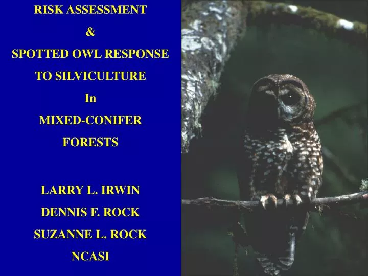
1. RISK ASSESSMENT & SPOTTED OWL RESPONSE TO SILVICULTURE In MIXED-CONIFER FORESTS LARRY L. IRWIN DENNIS F. ROCK SUZANNE L. ROCK NCASI .

2. NPS

3. LANDSCAPE STRATEGY REQUIRES IMPROVED UNDERSTANDING OF NSO HABITAT SELECTION

4. “HABITAT ISSUE” REMAINS UNSETTLED

6. ADULT OWL FECUNDITY VS. DAVIS-LINT H-S SCORE CLE WEN KLA WSR % Area w/Suitability Score > 40 (Based on Observations of Owls)

7. LIMITED EXPERIENCE WITH OWL RESPONSES TO HABITAT CHANGES FROM FUEL TREATMENTS OR THINNING

8. GOALS • EVALUATE OWL RESPONSE TO THINNING • MODEL OWL HABITAT SELECTION USING STRUCTURE & COMPOSITION • DEVELOP A RISK ASSESSMENT TOOL

9. CASE-STUDY RESPONSES TO SILVICULTURE (Approx. 20% of 1,000-ac areas; ~ 100-120 Sq. ft/ac)

10. Radio-Tracking

15. SPRINGFIELD, OR DOUGLAS-FIR THINS

16. CASE-STUDY OBSERVATIONS (16) • 1. Owls didn’t leave (1 left in fall, returned in spring) • Home ranges didn’t change • Frequent-use areas usually didn’t change • 4. Increased use in some units after thinning • Edges seemed to be used during treatments • Location may be important. More-detailed analysis soon…

18. Current Understanding of Habitat Selection Supported by Stand-level View of Seral Stages Or Cover Types Studies Identified: Type(s) Used > Available Type(s) Used > Other Types CATEGORICAL APPROACH

19. O P/Y M O

20. CHOICES MADE AT SCALE OF A PATCH-- PATTERNS OF USE & HOME RANGES “EMERGE”

21. MULTI-VARIATE APPROACH: VEGETATION Structure and Composition PHYSICAL FEATURES Riparian zones, Slope, Aspect .

22. MEASURED PATCH-SCALE VARIATION Geo-referenced Inventory Plots

23. DO PATCH-LEVEL CONDITIONS MATTER TO OWLS? IF SO, HOW TO “SCALE UP”?

24. ~ 250 OWLS RADIO-TAGGED ~ 35,000 TELEM POINTS ~ 70,000 HAB. PLOTS

25. 100 x 200m GRID OF INVENTORY PLOTS TO ESTIMATE AVAILABLE UNITS 1 YEAR’S TELEMETRY PROVIDES 1 SAMPLE OF USED PATCHES .

26. OBJECTIVE: RESOURCE SELECTION FUNCTION (RSF) MODEL  VALUES PROPORTIONAL TO PROBABILITY OF SELECTION OF A RESOURCE UNIT (…HERE, PATCH) TOOLS  IMPROVED CONSERVATION & HABITAT ASSESSMENTS .

27. DISCRETE-CHOICE RSF • Combine Individ. Samples  ΣPopulation level • EST. PROB. (Patch Selection)| CONDITIONS • SPATIALLY EXPLICIT PREDICTIONS

28. FACTORS MEASURED ABIOTIC ENVIRONMENT TOPOGRAPHY (Water), ELEVATION, ROADS, NEST DISTANCE, SLOPE, ASPECT VEGETATION TPA, BASAL AREA, CAN. COVER %, QMD, TPA x Diam Class, TPA & BA by Species UNDERSTORY SHRUBS, SNAGS, LOGS Model Selection Among Candidates

30. Factors Influencing Selection of Nest SitesMay Differ from Those Influencing Selection of Further Away

31. REPEATED PATTERNS: 5 AREAS (4MC ) DISTANCE TO NEST (-) TOPOGRAPHIC POSITION (Lower; RMZ) ASPECT (N/E in Driest Areas) FIR BASAL AREA {Total & Trees > 26”} Qd or Pseud. PONDEROSA PINE BA (-); S. PINE & CEDAR (+) HARDWOODS (+), UNDERSTORY SHRUBS (+) WINTER—LOW BASAL AREA (SHRUBFIELDS) BA TREES > 26-in * DIST. NEST (-) SMALLER DIAM. TREES, CWD, SNAGS (nsd) __________________________________________________

32. ______________STUDY AREA___________________ YREKAMEDFORDCHICOK-FALLS NEST DIST. -2.4 -7.7 -15.8 -3.2 STREAMS -7.3 -9.4 - 3.2 -2.1 ASPECT -0.1 0.0 -2.0 -1.8 LRG BASAL 6.0* 3.9* 3.8 2.6* LRG BASAL2 -2.7 -1.5 0.2 -0.9 LRG * NEST-D -3.7 -3.6 - 3.9 -1.9 SHRUB DENS 4.4 2.7 -- 2.9 P. PINE BASAL -1.9 -1.8 -2.0 1.2 HardWood BA 1.0 0.6 4.7 5.3 * Pseudo-threshold was competing model; Sugar Pine (+), Incense Cedar

35. RSF for CASPO, Including Basal Area of Hardwoods and FIR Trees)

36. RSF for Medford & Yreka Total Basal Area

37. Why is Selection for Patches w\Large Trees reduced w/Distance from Nest? Owl Sites vs. Random Landscape Locations, W. OR Meyer et al. 1998. Wildlife Monograph

40. WHAT THINGS MATTER TO OWLS?

41. RSF SUMMARY • SIZE & DENSITY MATTER (NON-LINEAR) • SCALE OF VIEW MATTERS • TREE SPP. COMPOSITION MATTERS • UNDERSTORY SHRUBS MATTER • LOCATION MATTERS • (ABIOTIC FACTORS)

42. OPT/THRESHOLD BASAL AREA + SHRUBS + HARDWOODS + RESPONSES TO THINNINGS SUGGEST … HABITAT QUALITY MAY BE ENHANCED

43. RSF MODEL APPLICATIONS • Estimate Short-term Site-specific Risk of Changing Tree Density & Composition. • Estimate Risk Across Landscape Under Alternative Strategies. • Predict Long-term Risk Over Time, Via Inventory, FVS • Link with Fire Risk Models

44. EXPONENTIAL RSF: e (z*) , where z* = β1DistNest + β2DistWater + β3log(Agte26+1) – β4SHRUBS+ …. Scaled to 1.0

45. NET CHANGE IS TOTAL AREA UNDER THE “SURFACE" APPLY RSF TO GEO-INVENTORY (2-5ha Pixels) AVERAGE OF ALL PIXELS IS ESTIMATE OF NET “VALUE”

46. Depending on location, large clearcut would reduce net or overall value (A); positive habitat modifications should increase it (B). B A

47. Use 2-5 acre pixels in GIS; Sum across plan area to Identify Possible Future Replacement Habitat; Grow via FVS .

48. Overlay with Probability of Ignition & Fire spread

49. IMPLICATIONS • 1. Owls may respond favorably to fuel treatments • 2. Habitat Quality Multi-factored • Topography, Shrubs, Composition, Large Trees, Hardwoods • 3. RSF  Improved assessment & conservation tool. • 4. Extrapolations from patches to landscape. • (Stand may not be the correct unit) • 5. Dynamic landscape? Embedded abiotic factors • 6. May need different conditions close to nests • 7. RSF may help in prioritization or identifying replacement