
Performance Issues in Non-Gaussian Filtering Problems
E N D
Presentation Transcript
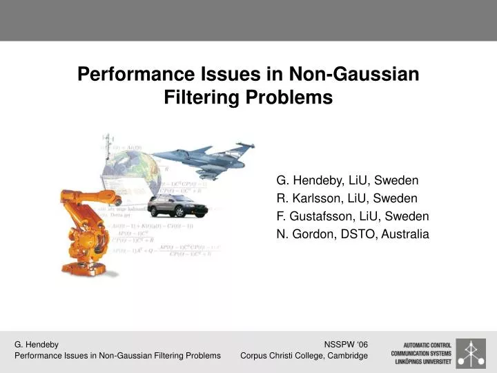
Performance Issues in Non-Gaussian Filtering Problems G. Hendeby, LiU, Sweden R. Karlsson, LiU, Sweden F. Gustafsson, LiU, Sweden N. Gordon, DSTO, Australia
Motivating Problem – Example I • Linear system: • non-Gaussian process noise • Gaussian measurement noise • Posterior distribution:distinctly non-Gaussian
Motivating Problem – Example II • Estimate target position based on two range measurements • Nonlinear measurements but Gaussian noise • Posterior distribution: bimodal
Filters The following filters have been evaluated and compared • Local approximation: • Extended Kalman Filter (EKF) • Multiple Model Filter (MMF) • Global approximation: • Particle Filter (PF) • Point Mass Filter (PMF, representing truth)
Filters: EKF EKF: Linearize the model around the best estimate and apply the Kalman filter (KF) to the resulting system.
Filter 1 Filter 1 Filter 1 Filter 1 Mix Filter 2 Filter 2 Filter M Filter M Filters: MMF • Run several EKF in parallel, and combine the results based on measurements and switching probabilities
Filters: PF Simulate several possible states and compare to the measurements obtained.
Filters: PMF • Grid the state space and propagate the probabilities according to the Bayesian relations
Filter Evaluation (1/2) Mean square error (MSE) • Standard performance measure • Approximates the estimate covariance • Bounded by the Cramér-Rao Lower Bound (CRLB) • Ignores higher-order moments!
Filter Evaluation (2/2) Kullback divergence • Compares the distance between two distributions • Captures all moments of the distributions
Filter Evaluation (2/2) Kullback divergence – Gaussian example • Let • The result depends on the normalized difference in mean and the relative difference in variance
Example I • Linear system: • non-Gaussian process noise • Gaussian measurement noise • Posterior distribution:distinctly non-Gaussian
Simulation results – Example I • MSE similar for both KF and PF! • KL is better for PF, which is accounted for by multimodal target distribution which is closer to the truth
Example II • Estimate target position based on two range measurements • Nonlinear measurements but Gaussian noise • Posterior distribution: bimodal
Simulation results – Example II (1/2) • MSE differs only slightly for EKF and PF • KD differs more, again since PF handles the non-Gaussian posterior distribution better
Simulation results – Example II (2/2) • Using the estimated position to determine the likelihood to be in the indicated region • The EKF based estimate differs substantially from the truth
Conclusions • MSE and Kullback divergence evaluated as performance measures • Important information is missed by the MSE, as shown in two examples • The Kullback divergence can be used as a complement to traditional MSE evaluation
Thanksforlistening Questions?