Get Folder
Get Folder. Network Neighbourhood Tcd.ie Ntserver-usr Get richmond. Books – Econophysics. Statistical Mechanics of Financial Markets J Voit Springer ISBN 3 540 41409 6 Patterns of Speculation; A study in Observational Econophysics BM Roehner Cambridge Introduction to Econophysics

Get Folder
E N D
Presentation Transcript
Get Folder • Network Neighbourhood • Tcd.ie • Ntserver-usr • Get • richmond SS 4013
Books – Econophysics • Statistical Mechanics of Financial Markets • J Voit Springer ISBN 3 540 41409 6 • Patterns of Speculation; A study in Observational Econophysics • BM Roehner Cambridge • Introduction to Econophysics • HE Stanley and R Mantegna Cambridge • Cambridge ISBN 0 521 62008 2 • Theory of Financial Risk: From Statistical Physics to Risk Management • JP Bouchaud & M Potters Cambridge • Financial Market Complexity • Johnson, Jefferies & Minh Hui Oxford SS 4013
Econophysics SS-4013Syllabus • What is a stock? • Reading the press; fundamental and noise traders • Price formation; market and limit orders; order book • Historical data; indices and price time series; price returns; volatility; fat tails • Distribution functions; • joint distributions; • Bayes’ theorem; conditional and unconditional distributions • Characteristic functions; normal distributions; Levy distributions; kurtosis; • combining random variables;central limit theorem; stable distributions; • Markov process; Chapman Kolmogorov; • Bachelier’s approach to price fluctuations; • Additive noise, Gaussian and Wiener random walks; multiplicative walks • Stochastic differential equations • Langevin Equations SS 4013
Breakdown of Bachelier and Gaussian – Empirical or Stylized facts • Distribution function for Returns • Scaling of financial data (price returns) • Mandelbrot; Stable Levy distributions • ‘Stanley’ data analysis for high frequency returns • Autocorrelation functions • Price returns • Clustered volatility SS 4013
Stock portfolios • Risk • Distribution functions; cumulative distributions • Gaussian v power laws • Minimizing risk • Markowicz’ theory and efficient market theory • Correlations • Stock taxonomy • Minimal spanning trees SS 4013
Options • Futures; calls and puts • Black Scholes SS 4013
Minority Game • El Farol problem • Bounded rationality SS 4013
Simple agent models • Model of Bouchaud Cont • Noise traders • Fundamental traders • Non linear effects: crashes and bubbles • Peer pressure and Lotka Volterra models • Can agents be modelled as molecules? SS 4013
2002 Exam 1 • A) How is a 1st order Markov process defined? [1] • Consider random variable x that takes values x1, x2, x3…..etc at times t1, t2, t3….etc • The probability for x1,t1 given the earlier sequence is • p(x1,t1|x2,t2, x3,t3…etc). • A first order Markov process is one where this probability distribution only depends on the previous value: ie p = p(x1,t1|x2,t2) • Generally just called a Markov process SS 4013
2 • B) The Chapman Kolmogorov equation is an integral equation for the conditional probability • p(x1,t1|x2,t2) = - p(x1,t1|x3,t3) p(x3,t3|x2,t2)dx3 • Explain how Bachelier used this equation to obtain a Gaussian distribution for stock price returns stating the assumptions used. You may ignore any complications due to Ito corrections. • Bachelier assumed • p(x1,t1|x2,t2) p(x1-x2,t1-t2|x2,t2) • He further assumed the fluctuations were independent. I.e. p(x1,t1|x2,t2) p(x1,t1) • CK equation now reduces to • p(x1,t1) = - p(x1-x3,t1-t3) p(x3,t3)dx3 • And can be solved with ansatz p(x,t) = p0(t)exp[-p02(t)x2) • This yields p02(t1+t2) = p02(t1) p02(t2)/ [ p02(t1) + p02(t2)] • p0(t) = H/t • Substitute 2 = t/2H2 • Obtain P(x,t) = exp[-x2/22(t)] / / 2(t) SS 4013
2 continued • Bachelier then identifies the random variable with the log of the asset price, S. • If this follows a random walk we have • S –S0 ~ (rt+)S ie lnS/S0 ~ rt + • Thus in expression for Gaussian • x = ln S/S0 – rt and (t) = t • This ignores the correction of Ito. With this correction included the correct expression is • X = ln S/S0 – {r -2/2}t • Hence distribution function for stock market returns of time horizon, t follows Gaussian distribution for all t. SS 4013
3 • How does distribution observed for stock price returns deviate from Gaussian? • Stock returns exhibit fat tailed distribution function. Modelled by Mandelbrot as Levy distribution with tail exponent of ~1.7. More recently Stanley et al have shown high frequency returns follow an exponent of ~4 (cumulative distribution ~3) SS 4013
4 • Bachelier assumes volatility, , to be constant. Sketch out how the volatility looks in practise • Volatility is |return| or an average of |return| over time. • Illustrative sketch for annual volatilities for FTA index over 19th and 20th centuries. Red line is constant assumed by Bachelier. SS 4013
5 • What is a market order? [1] • Market orders are executed immediately when a matching order(s) arrives irrespective of the stock price • The price may change during the waiting time • What is a limit order? [1] • A limit order is triggered when the market price reaches a predetermined threshold • Used to protect against unlimited losses or buying at too high a price • No guarantee exists that the order will be executed at or even close to the threshold SS 4013
162.2 6 • The pictures below are part of a market maker’s order book. Annotate the pictures explaining their meaning and show how the order is completed SS 4013
7 • How is the order book modified by the presence of a limit order? SS 4013
8 • Suppose orders arrive sequentially at random each with a mean waiting time of 3 minutes and standard deviation of 2 minutes. Consider the waiting time for 100 orders to arrive. What is the approximate probability that this will be greater than 400 minutes? • Assume events are independent. • For large number of events, use central limit theorem to obtain m and . • Thus • Mean waiting time, m, for 100 events is ~ 100*3 = 300 minutes • Average standard deviation, ~ 2/100 = 0.2 minutes • Model distribution by Gaussian, p(x) = 1/[(2)½] exp(-[x-m]2/22) • Answer required is • P(x>400) = 400 dx p(x) ~ 400 dx 1/((2)½) exp(-x2/22) • = 1/()½z dy exp(-y2) • where z = 400/0.04*2 ~ 7*10+3 • =1/2{ Erfc (7.103)} = ½ {1 – Erf (7.103)} • Information given: 2/ * z dy exp(-y2) = 1-Erf (x) • and tables of functions containing values for Erf(x) and or Erfc(x) SS 4013


