Download
1 / 36
380 likes | 512 Views
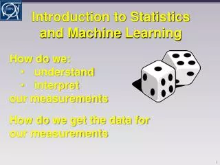
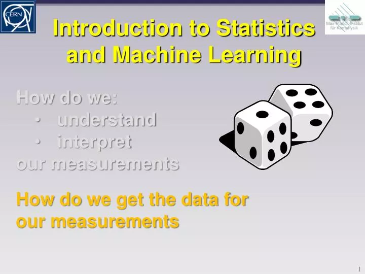
Introduction to Statistics and Machine Learning. How do we: understand interpret our measurements. How do we get the data for our measurements. Outline. Multivariate classification/regression algorithms (MVA) motivation

E N D
Introduction to Statisticsand Machine Learning • How do we: • understand • interpret • our measurements How do we get the data for our measurements
Outline • Multivariate classification/regression algorithms (MVA) • motivation • another introduction/repeat the ideas of hypothesis tests in this context • Multidimensional Likelihood (kNN: k-Nearest Neighbour) • Projective Likelihood (naïve Bayes) • What to do with correlated input variables? • Decorrelation strategies Introduction to Statistics and Machine Learning - GSI Power Week - Dec 5-9 2011
MVA-Literature /Software Packages... a biased selection Literature: • T.Hastie, R.Tibshirani, J.Friedman, “The Elements of Statistical Learning”, Springer 2001 • C.M.Bishop, “Pattern Recognition and Machine Learning”, Springer 2006 Software packages for Mulitvariate Data Analysis/Classification • individual classifier software • e.g. “JETNET” C.Peterson, T. Rognvaldsson, L.Loennblad and many other packages • attempts to provide “all inclusive” packages • StatPatternRecognition: I.Narsky, arXiv: physics/0507143 http://www.hep.caltech.edu/~narsky/spr.html • TMVA: Höcker,Speckmayer,Stelzer,Therhaag,von Toerne,Voss, arXiv: physics/0703039 http://tmva.sf.netor every ROOT distribution (development moved from SourceForge to ROOT repository) • WEKA: http://www.cs.waikato.ac.nz/ml/weka/ • “R”: a huge data analysis library: http://www.r-project.org/ Conferences: PHYSTAT, ACAT,… Introduction to Statistics and Machine Learning - GSI Power Week - Dec 5-9 2011
x2 x2 x2 S S S B B B x1 x1 x1 Event Classification • Suppose data sample of two types of events: with class labels Signal andBackground (will restrict here to two class cases. Many classifiers can in principle be extended to several classes, otherwise, analyses can be staged) • how to set the decision boundary to select events of type S? • we have discriminating variables x1, x2, … Rectangular cuts? A linear boundary? A nonlinear one? • How can we decide what to uses ? • Once decided on a class of boundaries, how to find the “optimal” one ? Low variance (stable), high bias methods High variance, small bias methods Introduction to Statistics and Machine Learning - GSI Power Week - Dec 5-9 2011
f(x) x x x Regression • how to estimate a “functional behaviour” from a given set of ‘known measurements” ? • assume for example “D”-variables that somehow characterize the shower in your calorimeter • energy as function of the calorimeter shower parameters . constant ? linear? non - linear? f(x) f(x) Energy Cluster Size • if we had an analytic model (i.e. know the function is a nth -order polynomial) than we know how to fit this (i.e. Maximum Likelihood Fit) • but what if we just want to “draw any kind of curve” and parameterize it? • seems trivial ? • seems trivial ? The human brain has very good pattern recognition capabilities! • what if you have many input variables? Introduction to Statistics and Machine Learning - GSI Power Week - Dec 5-9 2011
f(x,y) y x x Regression model functional behaviour • Assume for example “D”-variables that somehow characterize the shower in your calorimeter. • Monte Carlo or testbeam data sample with measured cluster observables + known particle energy = calibration function (energy == surface in D+1 dimensional space) 2-D example 1-D example f(x) events generated according: underlying distribution • better known: (linear) regression fit a known analytic function • e.g. the above 2-D example reasonable function would be: f(x) = ax2+by2+c • what if we don’t have a reasonable “model” ? need something more general: • e.g. piecewise defined splines, kernel estimators, decision trees to approximate f(x) NOT in order to “fit a parameter” provide predition of function value f(x) for new measurements x (where f(x) is not known) Introduction to Statistics and Machine Learning - GSI Power Week - Dec 5-9 2011
Find a mapping from D-dimensional input-observable =”feature” space to one dimensional output class label y(x) Event Classification • Each event, if Signal or Background, has “D” measured variables. y(x): RDR: D “feature space” most general form y = y(x); x D x={x1,….,xD}: input variables • plotting (historamming) the resulting y(x) values: • Who sees how this would look like for the regression problem? Introduction to Statistics and Machine Learning - GSI Power Week - Dec 5-9 2011
> cut: signal = cut: decision boundary < cut: background y(x): Event Classification • Each event, if Signal or Background, has “D” measured variables. • Find a mapping from D-dimensional input/observable/”feature” space to one dimensional output class lables y(B) 0, y(S) 1 y(x): RnR: D “feature space” • y(x): “test statistic” in D-dimensional space of input variables • distributions of y(x): PDFS(y) and PDFB(y) • used to set the selection cut! • efficiency and purity • y(x)=const: surface defining the decision boundary. • overlap of PDFS(y) and PDFB(y) separation power , purity Introduction to Statistics and Machine Learning - GSI Power Week - Dec 5-9 2011
Classification ↔ Regression Classification: • Each event, if Signal or Background, has “D” measured variables. • y(x): RDR: “test statistic” in D-dimensional space of input variables • y(x)=const: surface defining the decision boundary. D “feature space” y(x): RDR: Regression: • Each event has “D” measured variables + one function value (e.g. cluster shape variables in the ECAL + particles energy) • y(x): RDR find • y(x)=const hyperplanes where the target function is constant Now, y(x) needs to be build such that it best approximates the target, not such that it best separates signal from bkgr. f(x1,x2) X2 X1 Introduction to Statistics and Machine Learning - GSI Power Week - Dec 5-9 2011
1.5 0.45 y(x) Event Classification y(x): RnR: the mapping from the “feature space” (observables) to one output variable PDFB(y).PDFS(y): normalised distribution of y=y(x) for background and signal events (i.e. the “function” that describes the shape of the distribution) with y=y(x) one can also say PDFB(y(x)),PDFS(y(x)): : Probability densities for background and signal now let’s assume we have an unknown event from the example above for which y(x) = 0.2 PDFB(y(x)) = 1.5 and PDFS(y(x)) = 0.45 let fS and fB be the fraction of signal and background events in the sample, then: is the probability of an event with measured x={x1,….,xD} that gives y(x) to be of type signal Introduction to Statistics and Machine Learning - GSI Power Week - Dec 5-9 2011
Event Classification P(Class=C|x) (or simply P(C|x)) : probability that the event class is of C, given the measured observables x={x1,….,xD} y(x) Probability density distribution according to the measurements x and the given mapping function Prior probability to observe an event of “class C” i.e. the relative abundance of “signal” versus “background” Posterior probability Overall probability density to observe the actual measurement y(x). i.e. Introduction to Statistics and Machine Learning - GSI Power Week - Dec 5-9 2011
Any Decision Involves Risk! Decide to treat an event as “Signal” or “Background” Trying to select signal events: (i.e. try to disprove the null-hypothesis stating it were “only” a background event) Type-1 error: (false positive) classify event as Class C even though it is not (accept a hypothesis although it is not true/i.e.false) (reject the null-hypothesis although it would have been the correct one) • loss of purity (e.g. accepting wrong events) accept as: truly is: Type-2 error: (false negative) fail to identify an event from Class C as such (reject a hypothesis although it would have been correct/true) (fail to reject the null-hypothesis/accept null hypothesis although it is false) • loss of efficiency (e.g. miss true (signal) events) “A”: region of the outcome of the test where you accept the event as Signal: should be small Significance α: Type-1 error rate: α= background selection “efficiency” should be small Size β: Type-2 error rate: (how often you miss the signal) Power: 1- β = signal selection efficiency most of the rest of the lecture will be about methods that try to make as little mistakes as possible Introduction to Statistics and Machine Learning - GSI Power Week - Dec 5-9 2011
Neyman-Pearson Lemma “limit” in ROC curve given by likelihood ratio 1 Neyman-Peason: The Likelihood ratio used as “selection criterium” y(x) gives for each selection efficiency the best possible background rejection. i.e. it maximises the area under the “Receiver Operation Characteristics” (ROC) curve better classification y’(x) 1- ebackgr. good classification y’’(x) random guessing 0 esignal 0 1 varying y(x)>“cut” moves the working point (efficiency and purity) along the ROC curve how to choose “cut” need to know prior probabilities (S, Babundances) • measurement of signal cross section: maximum of S/√(S+B) or equiv. √(e·p) • discovery of a signal (typically: S<<B): maximum of S/√(B) • precision measurement: high purity (p) large background rejection • trigger selection: high efficiency (e) Introduction to Statistics and Machine Learning - GSI Power Week - Dec 5-9 2011
MVA and Machine Learning • The previous slide was basically the idea of “Multivariate Analysis” (MVA) • rem: What about “standard cuts” (event rejection in each variable separately with fix conditions. i.e. if x1>0 or x2<3 then background) ? • Finding y(x) : RnR • given a certain type of model class y(x) • in an automatic way using “known” or “previously solved” events • i.e. learn from known “patterns” • such that the resulting y(x) has good generalization properties when applied to “unknown” events (regression: fits well the target function “in between” the known training events that is what the “machine” is supposed to be doing: supervised machine learning • Of course… there’s no magic, we still need to: • choose the discriminating variables • choose the class of models (linear, non-linear, flexible or less flexible) • tune the “learning parameters” bias vs. variance trade off • check generalization properties • consider trade off between statistical and systematic uncertainties Introduction to Statistics and Machine Learning - GSI Power Week - Dec 5-9 2011
Event Classification • Unfortunately, the true probability densities functions are typically unknown: Neyman-Pearsons lemma doesn’t really help us directly • Monte Carlo simulation or in general cases: set of known (already classified) “events” • 2 different ways: Use these “training” events to: • estimate the functional form of p(x|C): (e.g. the differential cross section folded with the detector influences) from which the likelihood ratio can be obtained • e.g. D-dimensional histogram, Kernel densitiy estimators, … • find a “discrimination function” y(x) and corresponding decision boundary (i.e. hyperplane* in the “feature space”: y(x) = const) that optimially separates signal from background • e.g. Linear Discriminator, Neural Networks, … * hyperplane in the strict sense goes through the origin. Here I mean “affine set” to be precise Introduction to Statistics and Machine Learning - GSI Power Week - Dec 5-9 2011
Unsupervised Learning Just a short remark as we talked about “supervised” learning before: supervised: training with “events” for which we know the outcome (i.e. Signal or Backgr) un-supervised: - no prior knowledge about what is “Signal” or “Background” or … we don’t even know if there are different “event classes”, then you can for example do: - cluster analysis: if different “groups” are found class labels - principal component analysis: find basis in observable space with biggest hierarchical differences in the variance infer something about underlying substructure Examples: - think about “success” or “not success” rather than “signal” and “background” (i.e. a robot achieves his goal or does not / falls or does not fall/ …) - market survey: If asked many different question, maybe you can find “clusters” of people, group them together and test if there are correlations between this groups and their tendency to buy a certain product. address them specialy - medical survey: group people together and perhaps find common causes for certain diseases Introduction to Statistics and Machine Learning - GSI Power Week - Dec 5-9 2011
x2 • One expects to find in a volume V around point “x” N*∫P(x)dx events from a dataset with N events V h Kernel Density estimator of the probability density Nearest Neighbour and Kernel Density Estimator “events” distributed according to P(x) • estimate probability density P(x) in D-dimensional space: • The only thing at our disposal is our “training data” • Say we want to know P(x) at “this” point “x” “x” • For the chosen a rectangular volume K-events: x1 k(u): is called aKernel function • K (from the “training data”) estimate of average P(x) in the volume V: ∫P(x)dx = K/N V • Classification: Determine PDFS(x) and PDFB(x) • likelihood ratio as classifier! Introduction to Statistics and Machine Learning - GSI Power Week - Dec 5-9 2011
x2 • One expects to find in a volume V around point “x” N*∫P(x)dx events from a dataset with N events V h Nearest Neighbour and Kernel Density Estimator “events” distributed according to P(x) • estimate probability density P(x) in D-dimensional space: • The only thing at our disposal is our “training data” • Say we want to know P(x) at “this” point “x” “x” • For the chosen a rectangular volume K-events: x1 k(u): is called aKernel function: rectangular Parzen-Window • K (from the “training data”) estimate of average P(x) in the volume V: ∫P(x)dx = K/N V • Regression: If each events with (x1,x2) carries a “function value” f(x1,x2) (e.g. energy of incident particle) i.e.: the average function value Introduction to Statistics and Machine Learning - GSI Power Week - Dec 5-9 2011
x2 • One expects to find in a volume V around point “x” N*∫P(x)dx events from a dataset with N events V x2 h x1 Nearest Neighbour and Kernel Density Estimator “events” distributed according to P(x) • estimate probability density P(x) in D-dimensional space: • The only thing at our disposal is our “training data” • Say we want to know P(x) at “this” point “x” “x” • For the chosen a rectangular volume K-events: x1 • determine K from the “training data” with signal and background mixed together • kNN : k-Nearest Neighbours relative number events of the various classes amongst the k-nearest neighbours Introduction to Statistics and Machine Learning - GSI Power Week - Dec 5-9 2011
Kernel Density Estimator • Parzen Window: “rectangular Kernel” discontinuities at window edges • smoother model for P(x) when using smooth Kernel Functions: e.g. Gaussian ↔ probability density estimator averaged kernels individual kernels • place a “Gaussian” around each “training data point” and sum up their contributions at arbitrary points “x” P(x) • h: “size” of the Kernel “smoothing parameter” • there is a large variety of possible Kernel functions Introduction to Statistics and Machine Learning - GSI Power Week - Dec 5-9 2011
Kernel Density Estimator : a general probability density estimator using kernel K • h: “size” of the Kernel “smoothing parameter” • chosen size of the “smoothing-parameter” more important than kernel function • h too small: overtraining • h too large: not sensitive to features in P(x) • which metric for the Kernel (window)? • normalise all variables to same range • include correlations ? • Mahalanobis Metric: x*x xV-1x (Christopher M.Bishop) • a drawback of Kernel density estimators: Evaluation for any test events involves ALL TRAINING DATA typically very time consuming • binary search trees (i.e. Kd-trees) are typically used in kNN methods to speed up searching Introduction to Statistics and Machine Learning - GSI Power Week - Dec 5-9 2011
Bellman, R. (1961), Adaptive Control Processes: A Guided Tour, Princeton University Press. “Curse of Dimensionality” We all know: Filling a D-dimensional histogram to get a mapping of the PDF is typically unfeasable due to lack of Monte Carlo events. Shortcoming of nearest-neighbour strategies: • in higher dimensional classification/regression cases the idea of looking at “training events” in a reasonably small “vicinity” of the space point to be classified becomes difficult: consider: total phase space volume V=1D for a cube of a particular fraction of the volume: • In 10 dimensions: in order to capture 1% of the phase space 63% of range in each variable necessary that’s not “local” anymore.. • Therefore we still need to develop all the alternative classification/regression techniques Introduction to Statistics and Machine Learning - GSI Power Week - Dec 5-9 2011
PDFs discriminating variables Likelihood ratio for event event Classes: signal, background types Naïve Bayesian Classifier “often called: (projective) Likelihood” Multivariate Likelihood (k-Nearest Neighbour) estimate the full D-dimensional joint probability density product of marginal PDFs (1-dim “histograms”) If correlations between variables are weak: • One of the first and still very popular MVA-algorithm in HEP • No hard cuts on individual variables, • allow for some “fuzzyness”: one very signal like variable may counterweigh another less signal like variable • optimal method if correlations == 0 (Neyman Pearson Lemma) PDE introduces fuzzy logic Introduction to Statistics and Machine Learning - GSI Power Week - Dec 5-9 2011
event counting (histogramming) nonparametric fitting (i.e. splines,kernel) parametric (function) fitting Easy to automate, can create artefacts/suppress information Automatic, unbiased, but suboptimal Difficult to automate for arbitrary PDFs Naïve Bayesian Classifier “often called: (projective) Likelihood” How parameterise the 1-dim PDFs ?? example: original (underlying) distribution is Gaussian • If the correlations between variables is really negligible, this classifier is “perfect” (simple, robust, performing) • If not, you seriously loose performance • How can we “fix” this ? Introduction to Statistics and Machine Learning - GSI Power Week - Dec 5-9 2011
What if there are correlations? • Typically correlations are present: Cij=cov[ xi , x j ]=E[ xixj ]−E[ xi ]E[ xj ]≠0 (i≠j) pre-processing: choose set of linear transformed input variables for which Cij = 0 (i≠j) Introduction to Statistics and Machine Learning - GSI Power Week - Dec 5-9 2011
Decorrelation • Find variable transformation that diagonalises the covariance matrix • Determinesquare-rootC of correlation matrix C, i.e., C = C C • compute C by diagonalisingC: • transformation from original(x)in de-correlated variable space(x)by:x = C 1x Attention: eliminates only linear correlations!! Introduction to Statistics and Machine Learning - GSI Power Week - Dec 5-9 2011
Matrix of eigenvectors V obey the relation: PCA eliminates correlations! Decorrelation: Principal Component Analysis • PCA (unsupervised learning algorithm) • reduce dimensionality of a problem • find most dominant features in a distribution • Eigenvectors of covariance matrix “axis” in transformed variable space • large eigenvalue large variance along the axis (principal component) • sort eigenvectors according to their eigenvalues • transform dataset accordingly • diagonalised covariance matrix with first “variable” variable with largest variance sample means Principle Component (PC) of variablek eigenvector correlation matrix diagonalised square root of C Introduction to Statistics and Machine Learning - GSI Power Week - Dec 5-9 2011
How to Apply the Pre-Processing Transformation? • Correlation (decorrelation): different for signal and background variables • we don’t know beforehand if it is signal or background. • What do we do? • for likelihood ratio, decorrelate signal and background independently signal transformation background transformation • for other estimators, one needs to decide on one of the two… (or decorrelate on a mixture of signal and background events) Introduction to Statistics and Machine Learning - GSI Power Week - Dec 5-9 2011
Decorrelation at Work • Example: linear correlated Gaussians decorrelation works to 100% • 1-D Likelihood on decorrelated sample give best possible performance • compare also the effect on the MVA-output variable! correlated variables: after decorrelation (note the different scale on the y-axis… sorry) Introduction to Statistics and Machine Learning - GSI Power Week - Dec 5-9 2011
Limitations of the Decorrelation • in cases with non-Gaussian distributions and/or nonlinear correlations, the decorrelation needs to be treated with care • How does linear decorrelation affect cases where correlations between signal and background differ? Original correlations Signal Background Introduction to Statistics and Machine Learning - GSI Power Week - Dec 5-9 2011
Limitations of the Decorrelation • in cases with non-Gaussian distributions and/or nonlinear correlations, the decorrelation needs to be treated with care • How does linear decorrelation affect cases where correlations between signal and background differ? SQRT decorrelation Signal Background Introduction to Statistics and Machine Learning - GSI Power Week - Dec 5-9 2011
Limitations of the Decorrelation • in cases with non-Gaussian distributions and/or nonlinear correlations, the decorrelation needs to be treated with care • How does linear decorrelation affect strongly nonlinear cases ? Original correlations Signal Background Introduction to Statistics and Machine Learning - GSI Power Week - Dec 5-9 2011
Limitations of the Decorrelation • in cases with non-Gaussian distributions and/or nonlinear correlations, the decorrelation needs to be treated with care • How does linear decorrelation affect strongly nonlinear cases ? SQRT decorrelation Signal Background • Watch out before you used decorrelation “blindly”!! • Perhaps “decorrelate” only a subspace! Introduction to Statistics and Machine Learning - GSI Power Week - Dec 5-9 2011
“Gaussian-isation“ • Improve decorrelation by pre-Gaussianisation of variables • First: transformation to achieve uniform (flat) distribution: Rarity transform of variablek Measured value PDF of variable k • The integral can be solved in an unbinned way by event counting, or by creating non-parametric PDFs (see later for likelihood section) • Second: make Gaussian via inverse error function: • Third: decorrelate (and “iterate” this procedure) Introduction to Statistics and Machine Learning - GSI Power Week - Dec 5-9 2011
“Gaussian-isation“ Original Signal - Gaussianised Background - Gaussianised We cannot simultaneously “Gaussianise” both signal and background ! Introduction to Statistics and Machine Learning - GSI Power Week - Dec 5-9 2011
Summary • Hope you are all convinced that Multivariate Algorithem are nice and powerful classification techniques • Do not use hard selection criteria (cuts) on each individual observables • Look at all observables “together” • eg. combing them into 1 variable • Mulitdimensinal Likelihood PDF in D-dimensions • Projective Likelihood (Naïve Bayesian) PDF in D times 1 dimension • How to “avoid” correlations Introduction to Statistics and Machine Learning - GSI Power Week - Dec 5-9 2011