COHERENT RISKS
Alexander S. Cherny. COHERENT RISKS. AND THEIR APPLICATIONS. PLAN. Why are coherent risks needed? How are coherent risks used?. COHERENT RISKS. Artzner, Delbaen, Eber, Heath (1997) Definition. A coherent risk is a map r ( X ): (i) r ( X + Y ) b r ( X ) +r ( Y );

COHERENT RISKS
E N D
Presentation Transcript
Alexander S. Cherny COHERENT RISKS AND THEIR APPLICATIONS
PLAN • Why are coherent risks needed? • How are coherent risks used?
COHERENT RISKS Artzner, Delbaen, Eber, Heath (1997) Definition.A coherent risk is a map r(X): (i)r(X+Y) b r(X)+r(Y); (ii) If X b Y, then r(X) r r(Y); (iii)r(lX) = lr(X) for lr0; (iv)r(X+m) = r(X)-m for m. Theorem.ris a coherent risk r(X) = -minQDEQX. Probabilistic scenarios Terminal wealth of a portfolio
EXAMPLES Scenario-based risk:r(X) = -min{X(w1),…,X(wN)}, where N and w1,…,wN are possible scenarios. TV@R:r(X) = -E(X|Xbql), where l(0,1) andql is the l-quantile of X. XV@R:(27)r(X) = -Emin{X1,…,XN}, where N and X1,…,XNare independent copies of X. Numbers in green are the numbers of papers on my website: http://mech.math.msu.su/~cherny
OPERATIONS Maximum:r1,…,rN are coherent risks r(X)= max{r1(X),…,rN(X)} is a coherent risk with D = D1…DN. Conv. combination:r1,…,rN are coherent risks • r(X)=l1r1(X)+…+lNrN(X) is a coherent risk with D = l1D1+…+lNDN. Convolution:r1,…,rN are coherent risks r(X) = min{r1(X1)+…+rN(XN):X1+…+XN=X} is a coherent risk with D = D1… DN. (28)
FACTOR RISKS-I X-P&L of a portfolio over the unit time period F - increment of a market factor over this period Problem:Risk of X driven by F = ? Definition.(27)Factor risk of X driven by F: rf(X;F) =r(j(F)), where j(z) =E(X | F=z). This is a coherent risk with Df = {E(Z|F):ZD}.
FACTOR RISKS-II X = X1+…+Xd
FACTOR RISKS-II X = X1+…+Xd rf(X;F) = r(j(F)), where j(z) = j1(z)+…+jd(z), ji(z) = E(Xi|F=z). TV@R:rf(X;F) = -E(j(F)bql), where qlis the l-quantile of j(F).
FACTOR RISKS-II X = X1+…+Xd rf(X;F) = r(j(F)), where j(z) = j1(z)+…+jd(z), ji(z) = E(Xi|F=z). TV@R:rf(X;F) = -E(j(F)bql), where qlis the l-quantile of j(F).
FACTOR RISKS-II X = X1+…+Xd rf(X;F) = r(j(F)), where j(z) = j1(z)+…+jd(z), ji(z) = E(Xi|F=z). TV@R:rf(X;F) = -E(j(F)bql), where qlis the l-quantile of j(F). XV@R:rf(X;F) = -Emin{j(F1),…,j(FN)}, where F1,…,FNare independent copies of F.
COHERENT RISKS Artzner, Delbaen, Eber, Heath (1997) Definition.A coherent risk is a map r(X): (i)r(X+Y) b r(X)+r(Y); (ii) If X b Y, then r(X) r r(Y); (iii)r(lX) = lr(X) for lr0; (iv)r(X+m) = r(X)-m for m. Theorem.ris a coherent risk r(X) = -minQDEQX. Probabilistic scenarios Terminal wealth of a portfolio
COHERENT RISKS Artzner, Delbaen, Eber, Heath (1997) Definition.A coherent risk is a map r(X): (i)r(X+Y) b r(X)+r(Y); (ii) If X b Y, then r(X) r r(Y); (iii)r(lX) = lr(X) for lr0; (iv)r(X+m) = r(X)-m for m. Theorem.ris a coherent risk r(X) = -minQDEQX. Probabilistic scenarios Terminal wealth of a portfolio
V@R X=+1 with P=0.96 X=-100 with P=0.04 l=0.05 V@Rl(X)=-1 -76 !
COHERENT RISKS Artzner, Delbaen, Eber, Heath (1997) Definition.A coherent risk is a map r(X): (i)r(X+Y) b r(X)+r(Y); (ii) If X b Y, then r(X) r r(Y); (iii)r(lX) = lr(X) for lr0; (iv)r(X+m) = r(X)-m for m. Theorem.ris a coherent risk r(X) = -minQDEQX. Probabilistic scenarios Terminal wealth of a portfolio
COHERENT RISKS Artzner, Delbaen, Eber, Heath (1997) Definition.A coherent risk is a map r(X): (i)r(X+Y) b r(X)+r(Y); (ii) If X b Y, then r(X) r r(Y); (iii)r(lX) = lr(X) for lr0; (iv)r(X+m) = r(X)-m for m. Theorem.ris a coherent risk r(X) = -minQDEQX. Probabilistic scenarios Terminal wealth of a portfolio
QUADRATIC RISK-I Do you agree that these two positions have the same risk? Do you agree that the risk of any position coincides with the risk of the opposite position?
QUADRATIC RISK-II X=-1 with P=0.5 Y=-1 with P=0.5 X=+1 with P=0.5 Y=+0.5 with P=0.48 Y=+13 with P=0.02 EX=0 EY=0
QUADRATIC RISK-II X=-1 with P=0.5 Y=-1 with P=0.5 X=+1 with P=0.5 Y=+0.5 with P=0.48 Y=+13 with P=0.02 EX=0, VarX=1EY=0, VarY=7.75 Do you agree that Y is 7 times riskier than X?
QUADRATIC RISK-III r(X) = -EX+SvarX is a coherent risk But there exist better coherent risks!
APPLICATIONS Coherent risks provide a uniform basis for: • risk measurement, • capital allocation, • risk management, • pricing and hedging, • assessing trades.
CAPITAL ALLOCATION X – P&L earned by a company
CAPITAL ALLOCATION X = (X1+…+Xd) – P&L earned by a company Problem: How is the risk r(X) allocated between the desks? r(X1)+…+r(Xd)>r(X) – diversification! Definition.Risk contribution of Y to X: rc(Y;X) = -EQ*Y, where Q*=argminQDEQX. Capital allocation:rc(X1;X),…, rc(Xd;X). P&L of a subportfolio P&L of a portfolio
EXAMPLES Scenario-based risk:r(X) = -min{X(w1),…,X(wN)}, where N and w1,…,wN are possible scenarios. TV@R:r(X) = -E(X|Xbql), where l(0,1) andql is the l-quantile of X. XV@R:(27)r(X) = -Emin{X1,…,XN}, where N and X1,…,XNare independent copies of X. Numbers in green are the numbers of papers on my website: http://mech.math.msu.su/~cherny
RISK CONTRIBUTION Scenario-based risk:rc(Y;X) = -Y(wn*), where n*=argminn=1,…,NX(wn). TV@R:rc(Y;X) = -E(Y|Xbql), where qlis the l-quantile of X. XV@R:rc(Y;X) = -EYn*, where n*=argminn=1,…,NXn, (X1,Y1),…,(XN,YN) areindependent copies of (X,Y). Properties:rc(X1;X)+…+rc(Xd;X) = r(X), rc(Y;X) = lime0 e-1[r(X+eY)-r(X)], YX r(X+Y) r(X)+ rc(Y;X).
RISK CONTRIBUTION Scenario-based risk:rc(Y;X) = -Y(wn*), where n*=argminn=1,…,NX(wn). TV@R:rc(Y;X) = -E(Y|Xbql), where qlis the l-quantile of X. XV@R:rc(Y;X) = -EYn*, where n*=argminn=1,…,NXn, (X1,Y1),…,(XN,YN) areindependent copies of (X,Y). Properties:rc(X1;X)+…+rc(Xd;X) = r(X), rc(Y;X) = lime0 e-1[r(X+eY)-r(X)], YX r(X+Y) r(X)+ rc(Y;X).
RISK MANAGEMENT-I Problem:E(X1+…+Xd) max, XiAi – P&Ls available to the i-th desk, r(X1+…+Xd)bC- firm’s capital. Theorem. (25) If (X1,…,Xd) is optimal, then EX1/rc(X1;X) =…= EXd/rc(Xd;X), whereX = X1+…+Xd.
RISK MANAGEMENT-I Problem:E(X1+…+Xd) max, XiAi – P&Ls available to the i-th desk, r(X1+…+Xd)bC- firm’s capital. Theorem. (25) If (X1,…,Xd) is optimal, then EX1/rc(X1;X) =…= EXd/rc(Xd;X), RAROCc(X1 ; X) RAROCc(Xd ; X), whereX = X1+…+Xd.
RISK MANAGEMENT-II Question: Is it possible to decentralize the procedure of imposing risk limits? Yes! Theorem. (27) If the limits are imposed on the risk contributions and the desks are allowed to trade these limits within the firm, then the equilibrium is an optimal solution, and vice versa.
PRICING AND HEDGING F - contingent claim A – space of P&Ls of possible trading strategies Problem:Find x and XA such that r(X-F+x)b0 and x is as small as possible.
PRICING AND HEDGING F - contingent claim A – space of P&Ls of possible trading strategies Problem:Find x and XA such that r(X-F)bx and x is as small as possible. Price: minXAr(X-F) Hedge: argminXAr(X-F) Quadratic risk:P – pricing measure Price:EPF Hedge: argminXAVar(X-F) Risk-adjusted price:EPF+aVar(X*-F) Which r to apply?
PRICING AND HEDGING F - contingent claim A – space of P&Ls of possible trading strategies Problem:Find x and XA such that r(X-F)bx and x is as small as possible. Risk-adjusted price: minXAr(X-F) Hedge: argminXAr(X-F) Quadratic risk:P – pricing measure Price:EPF Hedge: argminXAVar(X-F) Risk-adjusted price:EPF+aVar(X*-F) Which r to apply?
Theorem.Ifr(Z)=-minQDEQZ, then rm(Z) := minXAr(X+Z) = -minQDREQZ, whereR={Q:EQX=0 XA}. Risk-adjusted price of F equals minXAr(X-F) = maxQDREQF = EQ*F W – P&L of the firm’s overall portfolio rm(W) = r(X*+W) = EQ**W rm(W-F) -EQ**W+EQ**F if FW Risk-adjusted price contribution of F to W equalsEQ**F, where Q** = argminQDREQW. Market-modified risk
Theorem.Ifr(Z)=-minQDEQZ, then rm(Z) := minXAr(X+Z) = -minQDREQZ, whereR={Q:EQX=0 XA}. Risk-adjusted price of F equals minXAr(X-F) = maxQDREQF = EQ*F W – P&L of the firm’s overall portfolio rm(W)= r(X*+W) = EQ**W rm(W-F) -EQ**W+EQ**F if FW Risk-adjusted price contribution of F to W equalsEQ**F, where Q**=argminQDREQW. Market-modified risk Risk
Theorem.Ifr(Z)=-minQDEQZ, then rm(Z) := minXAr(X+Z) = -minQDREQZ, whereR={Q:EQX=0 XA}. Risk-adjusted price of F equals minXAr(X-F) = maxQDREQF = EQ*F W – P&L of the firm’s overall portfolio rm(W)= r(X*+W) = EQ**W rm(W-F) -EQ**W+EQ**F if FW Risk-adjusted price contribution of F to W equalsEQ**F, where Q**=argminQDREQW. Market-modified risk Risk Hedge
Theorem.Ifr(Z)=-minQDEQZ, then rm(Z) := minXAr(X+Z) = -minQDREQZ, whereR={Q:EQX=0 XA}. Risk-adjusted price of F equals minXAr(X-F) = maxQDREQF = EQ*F W – P&L of the firm’s overall portfolio rm(W)= r(X*+W) = EQ**W rm(W-F) -EQ**W+EQ**F if FW Risk-adjusted price contribution of F to W equalsEQ**F, where Q**=argminQDREQW. Market-modified risk Risk Hedge Extreme measure
Theorem.Ifr(Z)=-minQDEQZ, then rm(Z) := minXAr(X+Z) = -minQDREQZ, whereR={Q:EQX=0 XA}. Risk-adjusted price of F equals minXAr(X-F) = maxQDREQF = EQ*F W – P&L of the firm’s overall portfolio rm(W)= r(X*+W) = EQ**W rm(W-F) -EQ**W+EQ**F if FW Risk-adjusted price contribution of F to W equalsEQ**F, where Q**=argminQDREQW. Market-modified risk Risk Hedge Extreme measure