Download
1 / 71
710 likes | 922 Views
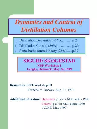
Dynamics and Control of Distillation Columns. Distillation Dynamics (45%)……….p.2 Distillation Control (30%)……….....p.23 Some basic control theory (25%)…..p.37. Revised for: NDF Workshop III Trondheim, Norway, Aug. 22, 1991 Additional Literature: Dynamics : p. 75 in NDF Notes 1990

E N D
Dynamics and Control of Distillation Columns • Distillation Dynamics (45%)……….p.2 • Distillation Control (30%)……….....p.23 • Some basic control theory (25%)…..p.37 Revised for: NDF Workshop III Trondheim, Norway, Aug. 22, 1991 Additional Literature: Dynamics: p. 75 in NDF Notes 1990 Control: p.57 in NDF Notes 1990 (AIChE, May 1990) SIGURD SKOGESTAD NDF Workshop I Lyngby, Denmark, May 24, 1989
1.4.1 Dominating time constant 8 1.1.4 Internal flows 17 2 • Distillation Dynamics • 1.1 Introduction 3 • 1.2 Degrees of freedom/steady state 4 • 1.3 Dynamic Equations 5 • 1.4 composition Dynamics7 • 1.5 Flow dynamics 19 • 1.6 Overall Dynamics 21 • 1.7 Nonlinearity 21A • 1.8 Linearization 22
3 1.1 IntroductionTypical column: 1 feed, 2 products, no intermediate cooling
MO, MB, P, YP, XB (5) Inventory Separation (composition, temperature) 3a Manipulated Variables (Valves): (μ) V (indirectly), L, D, B, VT (indirectly) (5) Disturbances: (d) F, zF, qF (= fraction liquid in feed, feed enthalpy), rain shower, + all u’s above Controlled Variables (y)
e.g., YD and xB Ttop and Tatm D (product rate) and YD etc. Recall specifications for steady-state simulations (PROCESS) 4 (1.2) STEADY-STATE OPERATION • Must keep holdups (MD,MB,MV) constant • This uses 3 degrees of freedom (u’s); only two left. • The two degrees of freedom may be used to specify two product specifications
Infinite reflux, exact (Fenske): holds for columns with feed at optimal location 4a Steady-state behavior (design) Overall separation, binary Finite reflux, good approximation: (slight modification of Jafarey, Douglas, McAvoy, 1979) Example: 3-Stage Column • Constant p • Constant holdup liquid and level • Negligible vapor h. • Constant molar flows • Constant α=10 • 2 Vicor stages + total condenser • Mi = 1 kmol (i = 1,2,3)
M2 L=3 C = 1kmol/min ZF=0.5 M2 V=3.5 M2 B = 0.5 XB = 0.1 yi 0.9000 0.5263 Stage Condenser Feedstage Reboiler i 1 2 3 Li 3.05 4.05 Vi 3.55 33.55 Xi 0.9000 0.4737 0.1000 Get: Total reflux: Actual column: Approximation: 4b D = 0.5 YD=0.9
i+1 L XL+1 V Yi B XB(x0) <1 <1 x1 = 0 4c
5 1.3 Dynamics of Distillation Columns Balance equations in Accumulated = in – out =D/DT (inventory) out Assumptions (always used) A1. Perfect mixing on all stages A2. Equilibrium between vapor on liquid on each stage (adjust total no. of stages to match actual column) A3. Neglect heat loss from column, neglect heat capacity of wall and trays Additional Assumptions (not always) A4. Neglect vapor holdup (Mvi ≈ 0) A5. Constant pressure (vapor holdup constant) A6. Flow dynamics immediate (Mvi constant) A8. Constant molar flow A9. Linear tray hydraulics
stage Mi+1 i+1 Li+1 Vi i Mi Vi-1 Li i-1 FLASH (Strongly Nonlimear) 6 Balance equation for stage without feed/side draw INDEP. DIFF. Component balance (index for component not Shown EQ.
Total balance (sum of component balances) Energy balance Tray Hydraulics (Algebraic) A9.Simplified (linearized): 6a τL: time constant for change in liquid holdup (≈2-10sek.) λ: effect of increase in vapor rate on L Li0,Mi0,Vi0: steady-state values (t=0). (ALGEBRAIC) Pressure drop: Δpi = f(Mi,Vi,…)
6b Numerical Solution (Integration) More details: p.82 in NDF Notes 1990 Moles of component on tray i Solution (at given time) Given value of state variable Perform constant nU-flash (given internal energy and phase split (MLi, Mvi), compositions (xi, yi), temperature, pressure (ρi), spec energy (hi, Vi) Compute Li and Vi from tray hydraulics and pressure drop relations 2. Simplified Approach, neglect vapor holdup (Mvi = 0) State Variables: (NL on each tray) Mole fraction total holdup → Xi → Mi (note: ni = Mixi)
6a.1 Solution: 1. Given value of state variables, guess pressure, Pi 2. Perform bubble point flash (given xi,pi) → yi,Ti, enthalpies 3. Compute Vi from energy balance (gives “index problem”: LHS (derivative) is known) Common simplification: Use dVi 1dt = dhil /dt from previous step. (Do not set d/dt (MiVi) ≈ 0 constant molar flows 4. Compute Li and Pi from tray hydraulics and pressure drop.
SUM: (NC independent differential equations) xN No. of components No. of trays 7 (1.4) Composition Dynamics Might expect very high-order complicated behavior. Surprise: The dominant composition dynamics is approximately 1 order! 100% time τ1 Fig. Response in YD to step change τ1: approximately independent of what we step (reflux, feed rate, boilup,…) and what and where we measure (YD, Ttop, Tbtm, etc,…)
∆X2(t) Dist.m: (matlab subroutine) Feed tray VLE 63% reboiler ∆X3(t) condenser ∆X1(t) Step in ZF from 0.50 50 0.51 τ1=4.5 min. Time (min) 7a • EXAMPLE: 3-stage column (see p.4B) • Neglect flow dynamics (Mu = 1 = constant) • 1 state on each tray • Constant molar flows (V2 = V3) Fig. Response for 3-stage column to feed composition change. Note: Composition change inside column much larger than at column ends. This is the main reason for the “slow” composition response
xi+1 i+1 i Mixi i-1 Where the linearized VLE-constant is 7b Composition Response of an Individual Tray Component material balance, tray i Assume the column is at steady-state, and consider the effect of an increase in xifi to xi+1+∆xi+1. Assume flows constant, and neglect interactions between the trays (yi-1: constant). In terms of deviation variables
7c Collecting ∆Ki terms we get a 1st order response with time constant Overall response time from top to bottom of column (neglecting “vapor” interactions) total HOLDUP Inside Column Example: 3-stage Column Conclusion: Do not yet correct overall response time (4.5 min) by simply adding together individual trays.
L xB LB LB θL xB 8 1.4.1 τ1Dominant Time Constant • Objectives: • Understand why overall response 1st order • Develop formula for τ1 • When does τ1 not apply? Assumptions: Use A1-A6 A4. Mvi is negligible (OK when pressure is low; at 10 bar Mvi will be about 10% of liquid holdup) A6. Flow dynamics much faster than composition dynamics. τ1 time Response to step change in reflux )This does not imply that flow dynamics are not important for composition control!) In particular, assume liquid holdup (Mi) constant
New Steady-State t= (subscript f=final) Df YDf D,YD D(t) YD(t) Ft ,zFt Ft ,zFt B,xB B(t) xB(t) t = 0 t > 0 t = Column at Steady-State at t ≤ 0 Something Happens at t = 0 (not steady-state) F1zF Bf xBf Assumption 6: D(t) = Df B(t) = Bf Component balance whole column;
5 10 Assumption A7. “All trays have some dynamic response”, that is, (4) Justification: Large interaction between trays because of liquid and vapor streams. (Reasonable if Substitute (4) into (3):
3. Only steady-state data needed! (+holdups) Need steady-state before (t=0) and after (t=∞) upset. 4. (5) applies to any given component 5. τ1 may be extremely large if both products pure (Reason: Numerator>>Denominator because compositions inside column change a lot, while product compositions change very little). 6. Limitation: τ1 Does not apply to changes in INTERNAL FLOWS ONLY, that is, L and V increase with ∆D=0 and ∆B=0. Reason: Denominator (τ)=0, (will find τ2<τ1!)q 11 Comments on τ1-Formula (5)
Compositions Flows with ZF=0.50 with ZF=0.51 Stage Condenser Feed Stage Reboiler i 1 2 3 Li 3.05 4.05 Vi 3.55 3.55 Xi Yi Xi Yi 0.9000 0.4737 0.900 0.1000 0.5263 0.9091 0.5001 0.9091 0.1109 0.5549 12 Example (Continued): Three-stage column Estimated Dominant Time Constant Excellent agreement with observed 4.5 minute Check of Assumption (7): “All trays have same dynamic response”(because of tray interactions)
Overall response time (incl. Tray interactions) Response time neglecting tray interactions Reasonable if
13 Example 2. Propane-propylene splitter • 110 theoretical stages • = 1.12 (relative volatility) • Assume constant molar flows • L/D = 19, D/F = 0.614 • Find τ 1 when ZF decreases from 0.65 to 0.60 All flows kept constant zF yD xB 0.65 0.995 0.100 0.714 0.60 0.958 0.030 0.495 Simulation 1 (t=0) Simulation 2 (t=∞ )
Response: 0.05 ΔyD .63 0 time 8h 10h 0 1h
Varies with oper. Cond! (ln is typically from 4 to 15) Columns with pure products IS is small 14 • τ1: Shortcut Formula • Make some simplifying assumptions which hold best for columns with • large reflux • pure products • Small changes • Binary separation (or use pseudobinary)
15 For small changes assume (*) applies. Have Reasonable agreement: NOTE: Contribution small from condenser because purity is high so absolute changes in compositions are small
τ1 Peak is large if both products are pure 1 Typical plot. May be derived from shortcut formula. • Conclusion: Time constant depends on operating conditions – mainly on purity of least pure product (IS). • Get “asymmetric” behavior: • a.) Least pure product gets purer: Time constant gets longer (slow response) • b.) Least pure product gets less pure: Time constant gets smaller (fast response) Example ΔZF “Fast” Pure getting pore “slow” time 16 Variation in τ1 with operating point
tray 0 COMP1 0 AB=ΔD AB=ΔD=0 Large effect on composition (large “gain”) Effect on composition obtained by assuming separation factor constant Small effect on composition (small “gain”) Effect on composition obtained by considering change in S: (“separation unchanged split changed”) (“separation changed split unchanged”) MAIN EFFECT ON COMPOSITION BY ADJUSTING D/F; “FINE TUNE” WITH INTERNAL FLOWS 17 (1.4.2) τ2 External and Internal Flows Steady -state Steady -state Steady -state COMP
ΔxB 63% ΔyD ΔxB 0 63% ΔyD 0 τ1 τ2 time time Dynamics External Flows Internal Flows Step ΔB = -ΔD Step ΔL = -ΔV • Conclusion: • Large S.S. effect • Slow (τ1) • Small S.S. Effect • Faster (τ2) Initial Response: Not as Different Recall: (see more accurate formulas in Skogestas & Morari, 1988 I E E C Res, 27, 1848-1862) For columns with pure products But: Derived when flow dynamics neglected (doubtful since τ2 is relatively small)
i+1 Li+1 Mi i Li 19 FLOW DYNAMICS (variations in liquid holdup neglected so far) A8. Constant molar flows A4. Neglect vapor holdup Total material balance becomes
Tray Hydraulics A9.: Assume simplified linear tray hydraulics = hydraulic time constant = effect on change in Vi on Li (vapor may push liquid off tray, λ>0.5: inverse response) 19a
ΔL N ΔLB t θL=N·τL 20 Consider Deviations from Initial Steady-State (Δli=Li-Lio,…) Then Consider response in LB to change in L: N tanks in series, each time constant τL ΔL ΔLB 0.5ΔL V ΔV ΔLB t θL=N·τL (“almost” a dead time) Response in LB to change in V: “Vapor pushes liquid off each tray” ΔV λ·ΔV 0
+ Liquid Flow Dynamics “Dead time” from top to bottom, θL 3 minute + Pressure dynamics + Top level – “ – + BTM level – “ – + Valve dynamics, + Heat transfer dynamics (V and Vt indirectly controlled) + Measurements Dynamics Depend on tuning of pressure and level controls. Typical time constant: 0.5 minute 0.2 minute 0.1 minute 21 1.6 Overall Dynamics Composition Dynamics Typical value External flows , τ1 250 min Internal flows , τ2 20 min Essential for control ! • Simplified Model • Describe each effect independently • “Add” together to give overall dynamics • (Alternative: Linearize all equations) • NOTE: Exact value of τ1 not important for control!
Light key component on tray i Heavy component May also be used for temperatures! Temp. Top of Column Temp. on Tray i Temp. BTM. Of Column 21A 1.7 Nonlinearity The dynamic response of distillation column is strongly nonlinear. However, simple logarithmic transformations counteract most of the nonlinearity. Xi+1 Xi tray More details: p.132-133 in NDF Notes 1991
nonlinear nonlinear Linear model Linear model Extremely non linear ∆xB ∆yD Log: Counteracts Nonlinearity -∆(n(1-yD) ∆ ln xB 21b Initial Response to 10% ∆L: (V constant) (Column A with Flow Dynamics)
22 1.8 Linearization • Need linear models for controller design • Obtain by • Put together simple models of individual effects (previous page) • Linearize non-linear model Given Tray Linearize, introduce deviation variables, simplification here: assume: i) const., ii) const. molar flows Li = Li+1 = L Vi-1= Vi = V
= + A Δx + B ΔL ΔV inputs State matrix (eigen values determine speed of response) Output matrix “states” (tray compositions) • Can derive transfer matrix G(12) + Equations for dMi/dt=…… 22a
23 (2) Distillation Control Multivariable vs. Single-Loop Control…25 Choice of Control Configurations…27 LV DV, L DB • Disturbance Sensitivity………….31 • Feedback Control Properties…….34 • One-Point • Two-Point • Implementation, Level Control…..35
Manipulated inputs, μ1s: L,V,D,B,UT Controlled outputs, Y1s: Mo, Mb, ,YD, xB COLUMN MD MB MV YD XB L V D B UT 5X5 24 Distillation Control
25 Controller Design • “Full” 5x5 multivariable controller? NO! • Instead use simpler scheme (decentralized control) • 3 single loops (PI, PID) for Md, MB, MV (levels and pressure) • There are now left two degrees of freedom for quality controller (keep YD and xB at desired values). • Design as two single loops or 2x2 controller (e.g. decoubler) PROBLEM 1: Choice of Control Configuration (Structure). Which two degrees of freedom should be left for equality control? (Same as choice inputs for level control ) PROBLEM 2: Design of Controllers i) Level controllers ii) Composition controllers remaining 2x2 system
Single Loops • Problem: Interactions (performance) • Advantage: Robustness • (2) Mi variable, for example, decoupler • Problem: Often not robust • (Sensitive to errors) 26 Options Composition Control • “No control” that is, manual operation (e.g. reflux L and boilup V are set manually by the operator • “One-point” control: One composition controlled automatically. (e.g. yD controlled with L using PI-controller, the other input is n manual, xB “floats”). Most common in industry, often necessary because of constraints. • “Two-point” control: Both compositions unclear feedback control. • $$! Potential for large economic savings. • (larger throughput, more products, less energy) Possible Controller (2x2)
27 Problem 1. • LV-configuration (“conventional”, “energy balance”, “indirect material-balance”) • Reflux L and boilup V used for composition control • Level control: • MD D • MB B • MV (P) VT (cooling) • DV-configuration (“(direct) material balance”) • because D is used • Level control: • MD L • MB B • 3) LB-configuration (“(direct) material balance”) • Level control: • MD D • MB V • L/D V/B-configuration (“double ratio”) • Level control: • MD both L and D (with L/D constant) • MB both V and B (with V/B constant)
Top of Column VT LS LC L+D D L LV-configuration LB-configuration VT DS LC L+D D DV-configuration DB-configuration L 28
VT LC C L+D D L Comment: Will usually use cascade control on inputs for composition control DIV (40)m Set manually or from composition controller (L/D)s With cascade using flow measurements (remove nonlinear valve characteristics No cascade (manipulated valve position) LS Lm P LS L L 28a
Previously rejected from steady-state considerations (Perry, 1973; Shinskey, 1984; Skogestad & Morari, 1987; Haggblom & Waller, 1988). Works because mass may be accumulated dynamically (change in liquid level) 30 DB(!!) (Finco & Luyben, 1989) BAD
31 DIFFERENCE BETWEEN CONFIGURATIONS • Disturbance sensitivity (“self regulating” properties) • Interactions between loops, etc. (feedback control properties) • Implementation level control 1. DISTURBANCE SENSITIVITY Fact: Composition are mainly dependent on D/F (external flows) should have D/F ZF High-purity columns: Composition extremely sensitive to small changes in D/F: Consequently: Disturbances which change D/F are “bad” The effect of a given disturbance on D/F depends on the configuration
32 EXAMPLE Configuration Disturbance ΔFV (increase in flow rate of vapor in feed) ΔV (increase in boilup) Optimal (see figures p. 29-30) More detailed: See Table 3 in Skogestad, “Disturbance rejection in distillation columns” CHEMDATA’88, Goteberg, June 1988. LP. 65 Literature for 1989 NDF) or p. 40.