Download

1 / 47
470 likes | 598 Views
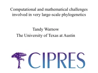
Computational and mathematical challenges involved in very large-scale phylogenetics. Tandy Warnow The University of Texas at Austin. How did life evolve on earth?. An international effort to understand how life evolved on earth

E N D
Computational and mathematical challenges involved in very large-scale phylogenetics Tandy Warnow The University of Texas at Austin
How did life evolve on earth? An international effort to understand how life evolved on earth Biomedical applications: drug design, protein structure and function prediction, biodiversity. • Courtesy of the Tree of Life project
Steps in a phylogenetic analysis • Gather data • Align sequences • Reconstruct phylogeny on the multiple alignment - often obtaining a large number of trees • Compute consensus (or otherwise estimate the reliable components of the evolutionary history) • Perform post-tree analyses.
Reconstructing the “Tree” of Life Handling large datasets: millions of species, and most problems are NP-hard Evolution is complex: Reticulate evolution Indels, genome rearrangements, etc. Gene tree/species tree differences
The CIPRES Project (Cyber-Infrastructure for Phylogenetic Research) The US National Science Foundation funds this project, which has the following major components: • ALGORITHMS and SOFTWARE: scaling to millions of sequences (open source, freely distributed) • MATHEMATICS/PROBABILITY/STATISTICS: Obtaining better mathematical theory under complex models of evolution • DATABASES: Producing new database technology for structured data, to enable scientific discoveries • SIMULATIONS: The first million taxon simulation under realistically complex models • OUTREACH: Museum partners, K-12, general scientific public • PORTAL available to all researchers • See www.phylo.org for more about CIPRES.
This talk • Part 1: Overview of some interesting mathematical issues • Part 2: Better heuristics for NP-hard optimization problems • Part 3: New methods for simultaneous estimation of trees and alignments • Part 4: Related research and open problems.
-3 mil yrs AAGACTT AAGACTT -2 mil yrs AAGGCCT AAGGCCT AAGGCCT AAGGCCT TGGACTT TGGACTT TGGACTT TGGACTT -1 mil yrs AGGGCAT AGGGCAT AGGGCAT TAGCCCT TAGCCCT TAGCCCT AGCACTT AGCACTT AGCACTT today AGGGCAT TAGCCCA TAGACTT AGCACAA AGCGCTT AGGGCAT TAGCCCA TAGACTT AGCACAA AGCGCTT DNA Sequence Evolution
Markov models of single site evolution Simplest (Jukes-Cantor): • The model tree is a pair (T,{e,p(e)}), where T is a rooted binary tree, and p(e) is the probability of a substitution on the edge e. • The state at the root is random. • If a site changes on an edge, it changes with equal probability to each of the remaining states. • The evolutionary process is Markovian. More complex models (such as the General Markov model) are also considered, often with little change to the theory.
Modelling variation between characters: Rates-across-sites • If a site (i.e., character) is twice as fast as another on one edge, it is twice as fast everywhere. • The distribution of the rates is typically assumed to be gamma. B D A C B D A C
Modelling variation between characters: The “no-common-mechanism” model • A separate random variable for every combination of site and edge - the underlying tree is fixed, but otherwise there are no constraints on variation between sites. C A D B B D A C
Identifiability and statistical consistency • A model is identifiable if it is uniquely characterized by the probability distribution it defines. • A phylogenetic reconstruction method is statistically consistent under a model if the probability that the method reconstructs the true tree goes to 1 as the sequence length increases.
Identifiability results • The “standard” Markov models (from Jukes-Cantor to the General Markov model) are identifiable. • These models are also identifiable when sites draw rates from a gamma distribution (easy to prove if the distribution is known, and harder to prove if the distribution must be estimated - cf.Allman’s talk). • However, mixed models are often not identifiable (cf. Matsen’s talk), nor are some models in which sites draw rates from more complex distributions. Phylogeny estimation typically is done under identifiable models.
What about phylogeny reconstruction methods? U V W X Y AGGGCAT TAGCCCA TAGACTT TGCACAA TGCGCTT X U Y V W
Local optimum Cost Global optimum Phylogenetic trees Phylogenetic reconstruction methods • Hill-climbing heuristics for NP-hard optimization criteria (Maximum Parsimony and Maximum Likelihood) • Polynomial time distance-based methods: Neighbor Joining, FastME, Weighbor, etc. • Bayesian methods
Performance criteria • Running time. • Space. • Statistical performance issues (e.g., statistical consistency and sequence length requirements) • “Topological accuracy” with respect to the underlying true tree. Typically studied in simulation. • Accuracy with respect to a particular criterion (e.g. tree length or likelihood score), on real data.
Quantifying Error FN FN: false negative (missing edge) FP: false positive (incorrect edge) 50% error rate FP
Statistical consistency, exponential convergence, and absolute fast convergence (afc)
Theoretical results: statistical consistency under typical models? • Neighbor Joining is polynomial time, and statistically consistent. • Maximum Parsimony is NP-hard, and even exact solutions are not statistically consistent. • Maximum Likelihood is NP-hard, but exact solutions are statistically consistent
Theoretical results: sequence length requirements under typical models? • Neighbor joining (and some other distance-based methods) will return the true tree with high probability provided sequence lengths are exponentialin the diameter of the tree (Erdos et al., Atteson). • Maximum likelihood will return the true tree with high probability provided sequence lengths are exponential in the number of taxa (Steel and Szekely).
Neighbor joining has poor performance on large diameter trees [Nakhleh et al. ISMB 2001] Simulation study based upon fixed edge lengths, K2P model of evolution, sequence lengths fixed to 1000 nucleotides. Error rates reflect proportion of incorrect edges in inferred trees. 0.8 NJ 0.6 Error Rate 0.4 0.2 0 0 400 800 1200 1600 No. Taxa
DCM1 Warnow, St. John, and Moret, SODA 2001 • A two-phase procedure which reduces the sequence length requirement of methods. The DCM phase produces a collection of trees, and the SQS phase picks the “best” tree. • The “base method” is applied to subsets of the original dataset. When the base method is NJ, you get DCM1-NJ. Exponentially converging method Absolute fast converging method DCM SQS
DCM1-boosting distance-based methods[Nakhleh et al. ISMB 2001] • Theorem: DCM1-NJ converges to the true tree from polynomial length sequences 0.8 NJ DCM1-NJ 0.6 Error Rate 0.4 0.2 0 0 400 800 1200 1600 No. Taxa
However, • The best accuracy in simulation tends to be from computationally intensive methods (and most molecular phylogeneticists prefer these methods). • Unfortunately, these approaches can take weeks or more, just to reach decent local optima. • Conclusion: We need better heuristics!
Part 2: Improved heuristics for NP-hard optimization problems
Local optimum Cost Global optimum Phylogenetic trees Approaches for “solving” MP/ML • Hill-climbing heuristics (which can get stuck in local optima) • Randomized algorithms for getting out of local optima • Approximation algorithms for MP (based upon Steiner Tree approximation algorithms).
Problems with current techniques for MP Shown here is the performance of a TNT heuristic maximum parsimony analysis on a real dataset of almost 14,000 sequences. (“Optimal” here means best score to date, using any method for any amount of time.) Acceptable error is below 0.01%. Performance of TNT with time
Observations • The best MP heuristics cannot get acceptably good solutions within 24 hours on some large datasets. • Datasets of these sizes may need months (or years) of further analysis to reach reasonable solutions. • Apparent convergence can be misleading.
Rec-I-DCM3: a new technique (Roshan et al.) • Combines a new decomposition technique (DCM3) with recursion and iteration, to produce a novel approach for escaping local optima • Tested initially on MP (maximum parsimony), but also implemented for ML and other optimization problems
Input: Set S of sequences, and guide-tree T 1. Compute short subtree graph G(S,T), based upon T 2. Find clique separator in the graph G(S,T) and form subproblems The DCM3 decomposition • DCM3 decompositions • can be obtained in O(n) time (the • short subtree graph is triangulated) • (2) yield small subproblems • (3) can be used iteratively
Iterative-DCM3 T DCM3 Base method T’
Rec-I-DCM3 significantly improves performance (Roshan et al.) Current best techniques DCM boosted version of best techniques Comparison of TNT to Rec-I-DCM3(TNT) on one large dataset
Observations • Rec-I-DCM3 improves upon the best performing heuristics for MP. • The improvement increases with the difficulty of the dataset. Rec-I-DCM3 also improves maximum likelihood (using RAxML) analyses (data not shown), and is included in the CIPRES portal.
Steps in a phylogenetic analysis • Gather data • Align sequences • Reconstruct phylogeny on the multiple alignment - often obtaining a large number of trees • Compute consensus (or otherwise estimate the reliable components of the evolutionary history) • Perform post-tree analyses.
Steps in a phylogenetic analysis • Gather data • Align sequences • Reconstruct phylogeny on the multiple alignment - often obtaining a large number of trees • Compute consensus (or otherwise estimate the reliable components of the evolutionary history) • Perform post-tree analyses.
Basic observations about standard two-phase methods • Many new MSA methods improve on ClustalW, with ProbCons and MAFFT the two best MSA methods. • Although alignment accuracy correlates with phylogenetic accuracy, it has less effect than might be expected (Wang et al., unpublished).
What about simultaneous estimation? • Several Bayesian methods for simultaneous estimation of trees and alignments have been developed, but none can be applied to datasets with more than (approx.) 20 sequences. • POY attempts to solve the NP-hard “minimum length tree” problem, where gaps contribute to the length of the tree and can be applied to large datasets. However, its performance on simulated data isn’t competitive with the best two-phase methods (unpublished data).
New method: SATe (Simultaneous Alignment and Tree estimation) • Developers: Warnow, Linder, Liu, Nelesen, and Zhao. • Basic technique: propose alignments (using treelength under a selected affine gap penalty), and compute maximum likelihood trees for these alignments under GTR. • Unpublished.
Simulation study • 100 taxon model trees (generated by r8s and then modified, so as to deviate from the molecular clock). • DNA sequences evolved under ROSE (indel events of blocks of nucleotides, plus HKY site evolution). The root sequence has 1000 sites. • We vary the gap length distribution, probability of gaps, and probability of substitutions, to produce 8 model conditions: models 1-4 have “long gaps” and 5-8 have “short gaps”. • We compared RAxML on various alignments (including the true alignment) to SATe.
Topological accuracy FN (false negative): proportion of correct edges missing from the estimated tree FP (false positive): proportion of incorrect edges in the estimated tree
Alignment accuracy • Normalized number of columns in the estimated alignment relative to the true alignment.
Alignment accuracy FN: proportion of correctly homologous pairs of nucleotides missing from the estimated alignment (i.e., 1-SP score). FP: proportion of incorrect pairings of nucleotides in the estimated alignment.
Other observations • SATe is more accurate at estimating the number of gaps and the correct alignment length than other methods. • The standard alignment accuracy measure, SP, is not particularly predictive of phylogenetic accuracy. • We still need methods for MSA under models that include rearrangements and duplications.
Part IV: Open questions • Tree shape (including branch lengths) has an impact on phylogeny reconstruction - but what model of tree shape to use? • What is the sequence length requirement for Maximum Likelihood? (Current bound is probably too large.) • Why is MP not so bad? • How to detect and reconstruct reticulate evolution? • “Teasing apart” trees under complex models? • What complex models are identifiable?
General comments • Current models of sequence evolution are clearly too simple, and more realistic ones are not identifiable. • Relative performance between methods can change as the models become more complex or as the number of taxa increases. • We do not know how methods perform under realistic conditions (nor how long we need to let computationally intensive methods run).
Acknowledgements • Funding: NSF, The David and Lucile Packard Foundation, The Program in Evolutionary Dynamics at Harvard, and The Institute for Cellular and Molecular Biology at UT-Austin. • Collaborators: Peter Erdos, Daniel Huson, Randy Linder, Kevin Liu, Bernard Moret, Serita Nelesen, Usman Roshan, Mike Steel, Katherine St. John, Laszlo Szekely, Tiffani Williams, and David Zhao.