Download

1 / 31
310 likes | 445 Views
Computational and mathematical challenges involved in very large-scale phylogenetics. Tandy Warnow The University of Texas at Austin. Species phylogeny. From the Tree of the Life Website, University of Arizona. Orangutan. Human. Gorilla. Chimpanzee. How did life evolve on earth?.

E N D
Computational and mathematical challenges involved in very large-scale phylogenetics Tandy Warnow The University of Texas at Austin
Species phylogeny From the Tree of the Life Website,University of Arizona Orangutan Human Gorilla Chimpanzee
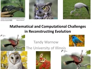
How did life evolve on earth? An international effort to understand how life evolved on earth Biomedical applications: drug design, protein structure and function prediction, biodiversity Phylogenetic estimation is a “Grand Challenge”: millions of taxa, NP-hard optimization problems • Courtesy of the Tree of Life project
-3 mil yrs AAGACTT AAGACTT -2 mil yrs AAGGCCT AAGGCCT AAGGCCT AAGGCCT TGGACTT TGGACTT TGGACTT TGGACTT -1 mil yrs AGGGCAT AGGGCAT AGGGCAT TAGCCCT TAGCCCT TAGCCCT AGCACTT AGCACTT AGCACTT today AGGGCAT TAGCCCA TAGACTT AGCACAA AGCGCTT AGGGCAT TAGCCCA TAGACTT AGCACAA AGCGCTT DNA Sequence Evolution
Step 1: Gather data S1 = AGGCTATCACCTGACCTCCA S2 = TAGCTATCACGACCGC S3 = TAGCTGACCGC S4 = TCACGACCGACA
Step 2: Multiple Sequence Alignment S1 = AGGCTATCACCTGACCTCCA S2 = TAGCTATCACGACCGC S3 = TAGCTGACCGC S4 = TCACGACCGACA S1 = -AGGCTATCACCTGACCTCCA S2 = TAG-CTATCAC--GACCGC-- S3 = TAG-CT-------GACCGC-- S4 = -------TCAC--GACCGACA
Step 3: Construct tree S1 = AGGCTATCACCTGACCTCCA S2 = TAGCTATCACGACCGC S3 = TAGCTGACCGC S4 = TCACGACCGACA S1 = -AGGCTATCACCTGACCTCCA S2 = TAG-CTATCAC--GACCGC-- S3 = TAG-CT-------GACCGC-- S4 = -------TCAC--GACCGACA S1 S2 S4 S3
Standard problem: Maximum Parsimony (Hamming distance Steiner Tree) • Input: Set S of n aligned sequences of length k • Output: A phylogenetic tree T • leaf-labeled by sequences in S • additional sequences of length k labeling the internal nodes of T such that is minimized.
Maximum parsimony (example) • Input: Four sequences • ACT • ACA • GTT • GTA • Question: which of the three trees has the best MP scores?
Maximum Parsimony ACT ACT ACA GTA GTT GTT ACA GTA GTA ACA ACT GTT
Maximum Parsimony ACT ACT ACA GTA GTT GTA ACA ACT 2 1 1 3 3 2 GTT GTT ACA GTA MP score = 7 MP score = 5 GTA ACA ACA GTA 2 1 1 ACT GTT MP score = 4 Optimal MP tree
Optimal labeling can be computed in linear time O(nk) GTA ACA ACA GTA 2 1 1 ACT GTT MP score = 4 Finding the optimal MP tree is NP-hard Maximum Parsimony: computational complexity
Local optimum Cost Global optimum Phylogenetic trees Approaches for “solving” MP (and other NP-hard problems in phylogeny) • Hill-climbing heuristics (which can get stuck in local optima) • Randomized algorithms for getting out of local optima • Approximation algorithms for MP (based upon Steiner Tree approximation algorithms).
Problems with current techniques for MP Shown here is the performance of a TNT heuristic maximum parsimony analysis on a real dataset of almost 14,000 sequences. (“Optimal” here means best score to date, using any method for any amount of time.) Acceptable error is below 0.01%. Performance of TNT with time
FN FN: false negative (missing edge) FP: false positive (incorrect edge) 50% error rate FP
Performance criteria • Estimated alignments are evaluated with respect to the true alignment. Studied both in simulation and on real data. • Estimated trees are evaluated for “topological accuracy” with respect to the true tree. Typically studied in simulation. • Methods for these problems can also be evaluated with respect to an optimization criterion (e.g., maximum likelihood score) as a function of running time. Typically studied on real data. (Reasonably valid for phylogeny but not yet for alignment.) Issues: Simulation studies need to be based upon realistic models, and “truth” is often not known for real data.
Statistical consistency, exponential convergence, and absolute fast convergence (afc)
Theorem: Neighbor joining (and some other distance-based methods) will return the true tree with high probability provided sequence lengths are exponentialin the diameter of the tree (Erdos et al., Atteson).
Neighbor joining has poor performance on large diameter trees [Nakhleh et al. ISMB 2001] Simulation study based upon fixed edge lengths, K2P model of evolution, sequence lengths fixed to 1000 nucleotides. Error rates reflect proportion of incorrect edges in inferred trees. 0.8 NJ 0.6 Error Rate 0.4 0.2 0 0 400 800 1200 1600 No. Taxa
Observations • The best current multiple sequence alignment methods can produce highly inacccurate alignments on large datasets (with the result that trees estimated on these alignments are also inaccurate). • The fast (polynomial time) methods produce highly inaccurate trees for many datasets. • Heuristics for NP-hard optimization problems often produce highly accurate trees, but can take months to reach solutions on large datasets.
Meta-algorithms for phylogenetics • Basic technique: determine the conditions under which a phylogeny reconstruction method does well (or poorly), and design a divide-and-conquer strategy to improve the performance • The divide-and-conquer technique is specific to the method.
Graph-theoretic divide-and-conquer (DCM’s) • Define a triangulated (i.e. chordal) graph so that its vertices correspond to the input taxa • Compute a decomposition of the graph into overlapping subgraphs, thus defining a decomposition of the taxa into overlapping subsets. • Apply the “base method” to each subset of taxa, to construct a subtree • Merge the subtrees into a single tree on the full set of taxa.
DCM1-boosting distance-based methods[Nakhleh et al. ISMB 2001] • Theorem: DCM1-NJ converges to the true tree from polynomial length sequences 0.8 NJ DCM1-NJ 0.6 Error Rate 0.4 0.2 0 0 400 800 1200 1600 No. Taxa
Input: Set S of sequences, and guide-tree T 1. Compute short subtree graph G(S,T), based upon T 2. Find clique separator in the graph G(S,T) and form subproblems The DCM3 decomposition • DCM3 decompositions • can be obtained in O(n) time (the • short subtree graph is triangulated) • (2) yield small subproblems • (3) can be used iteratively
Iterative-DCM3 T DCM3 Base method T’
Rec-I-DCM3 significantly improves performance (Roshan et al.) Current best techniques DCM boosted version of best techniques Comparison of TNT to Rec-I-DCM3(TNT) on one large dataset
Other problems • Multiple sequence alignment • Horizontal gene transfer (and other types of reticulation) detection and reconstruction • Inferring species trees from gene trees • Whole genome phylogenies • Reconstructing evolutionary histories of languages
For more information • My webpage: www.cs.utexas.edu/users/tandy • The CIPRES webpage www.phylo.org • Historical linguistics: www.cs.rice.edu/~nakhleh/CPHL
“Perfect Phylogenetic Network” (all characters compatible)