Importance of Data Pre-processing in Data Analysis
Learn the importance of pre-processing data to handle incomplete, noisy, and inconsistent data, and improve data quality for effective data analysis. Understand the reasons behind incomplete and noisy data, and discover data cleaning strategies for better mining outcomes.

Importance of Data Pre-processing in Data Analysis
E N D
Presentation Transcript
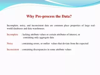
Why Pre-process the Data? Incomplete, noisy, and inconsistent data are common place properties of large real-world databases and data warehouses. Incomplete : lacking attribute values or certain attributes of interest, or containing only aggregate data Noisy : containing errors, or outlier values that deviate from the expected Inconsistent : containing discrepancies in some attribute values
Why Pre-process the Data? Incomplete data can occur for a number of reasons: Attributes of interest may not always be available, such as customer information for sales transaction data. Other data may not be included simply because it was not considered important at the time of entry. Relevant data may not be recorded due to a misunderstanding, or because of equipment malfunctions.
Why Pre-process the Data? There are many possible reasons for noisy data : The data collection instruments used may be faulty. There may have been human or computer errors occurring at data entry. Errors in data transmission can also occur. There may be technology limitations, such as limited buffer size for coordinating synchronized data transfer and consumption. Incorrect data may also result from inconsistencies in naming conventions or data codes used, or inconsistent formats for input fields, such as date.
Why Pre-process the Data? • If users believe the data are dirty, they are unlikely to trust the results of any data mining that has been applied to it. • Furthermore, dirty data can cause confusion for the mining procedure, resulting in unreliable output. • Although most mining routines have some procedures for dealing with incomplete or noisy data, they are not always robust.
Pre-process the Data Data cleaning routines work to “clean” the data by filling in missing values, smoothing noisy data, identifying or removing outliers, and resolving inconsistencies suppose that you would like to include data from multiple sources in your analysis. This would involve integrating multiple databases, data cubes, or files, that is, data integration . At the same time attributes representing a given concept may have different names in different databases, causing inconsistencies and redundancies. In addition to data cleaning, steps must be taken to help avoid redundancies during data integration.
Pre-process the Data If you would like to use a distance-based mining algorithm for your analysis, such as neural networks, nearest-neighbour classifiers, or clustering. Such methods provide better results if the data to be analyzed have been normalized, that is, scaled to a specific range such as [0.0, 1.0]. Data transformation operations, such as normalization and aggregation, are additional data preprocessing procedures that would contribute toward the success of the mining process.
Pre-process the Data • Data reduction obtains a reduced representation of the data set that is much smaller in volume, yet produces the same (or almost the same) analytical results. • The data set selected for analysis is HUGE, which is sure to slow down the mining process. • There are a number of strategies for data reduction: • data aggregation (e.g., building a data cube) • attribute subset selection ( e.g., removing irrelevant attributes through correlation • analysis) • dimensionality reduction(e.g., using encoding schemes such as minimum length encoding or wavelets)
Data Cleaning • Real-world data tend to be incomplete, noisy, and inconsistent. • Data cleaning (or data cleansing) routines attempt to fill in missing values, smooth out noise while identifying outliers, and correct inconsistencies in the data. • Missing Values • Many tuples have no recorded value for several attributes, such as customer income. • Ignore the tuple: • This is usually done when the class label is missing (assuming the mining task involves classification). • This method is not very effective, unless the tuple contains several attributes with missing values.
Data Cleaning Missing Values Fill in the missing value manually: In general, this approach is time-consuming and may not be feasible given a large data set with many missing values. Use a global constant to fill in the missing value: Replace all missing attribute values by the same constant, such as a label like “Unknown” or -∞. If missing values are replaced by, say, “Unknown,” then the mining program may mistakenly think that they form an interesting concept, since they all have a value in common—that of “Unknown.” Hence, although this method is simple, it is not foolproof.
Data Cleaning Missing Values Use the attribute mean to fill in the missing value: For example, suppose that the average income of AllElectronics customers is $56,000. Use this value to replace the missing value for income. Use the attribute mean for all samples belonging to the same class as the given tuple: For example, if classifying customers according to credit risk Replace the missing value with the average income value for customers in the same redit risk category as that of the given tuple.
Data Cleaning Missing Values It is important to note that, in some cases, a missing value may not imply an error in the data! For example, when applying for a credit card, candidates may be asked to supply their driver’s license number. Candidates who do not have a driver’s license may naturally leave this field blank. Hence, although we can try our best to clean the data after it is seized, good design of databases and of data entry procedures should help minimize the number of missing values or errors in the first place.
Data Cleaning Noisy Data “What is noise?” - Noise is a random error or variance in a measured variable. Given a numerical attribute such as, say, price, how can we “smooth” out the data to remove the noise? Binning: Binning methods smooth a sorted data value by consulting its “neighbourhood,” that is, the values around it. The sorted values are distributed into a number of “buckets,” or bins. In smoothing by bin means, each value in a bin is replaced by the mean value of the bin.
Data Cleaning In smoothing by bin medians each bin value is replaced by the bin median. In smoothing by bin boundaries, the minimum and maximum values in a given bin are identified as the bin boundaries.
Data Cleaning Noisy Data Regression: is a statistical process for estimating the relationships among variables. Data can be smoothed by fitting the data to a function, such as with regression. Linear regression involves finding the “best” line to fit two attributes (or variables), so that one attribute can be used to predict the other. Multiple linear regression is an extension of linear regression, where more than two attributes are involved and the data are fit to a multidimensional surface.
Data Cleaning Noisy Data Clustering: Outliers may be detected by clustering, where similar values are organized into groups, or “clusters.” Intuitively, values that fall outside of the set of clusters may be considered outliers .
Data Cleaning Data Cleaning as a Process : The first step in data cleaning as a process is discrepancy detection. Discrepancies can be caused by several factors, including : Poorly designed data entry forms that have many optional fields Human error in data entry Deliberate errors (e.g., respondents not wanting to disclose information about themselves) Data decay (e.g., outdated addresses).
Data Cleaning • Data Cleaning as a Process : • Discrepancies can be caused by several factors, including • Errors in instrumentation devices that record data, and system errors, are another source of discrepancies. • Errors can also occur when the data are (inadequately) used for purposes other than originally intended. • There may also be inconsistencies due to data integration (e.g., where a given attribute can have different names in different databases).
Data Cleaning • Data Cleaning as a Process : • How to identify the discrepancies? • Use meta data ( knowledge regarding properties of the data,) to identify discrepancies. • For example: • What are the domain and data type of each attribute? • What are the acceptable values for each attribute? • What is the range of the length of values? Do all values fall within the expected range? • Are there any known dependencies between attributes? • As a data analyst, you should examine inconsistent data representations such as “2004/12/25” and “25/12/2004” for date.
Data Cleaning • The data should also be examined regarding: • A unique rule says that each value of the given attribute must be different from all other values for that attribute. • A consecutive rule says that there can be no missing values between the lowest and highest values for the attribute, and that all values must also be unique (e.g., as in check numbers). • A null rule specifies the use of blanks, question marks, special characters, or other strings that may indicate the null condition (e.g., where a value for a given attribute is not available), and how such values should be handled.
Data Cleaning • There are a number of different commercial tools that can aid in the step of discrepancy detection. • Data scrubbing tools use simple domain knowledge (e.g., knowledge of postal addresses, and spell-checking) to detect errors and make corrections in the data. • Data auditing tools find discrepancies by analyzing the data to discover rules and relationships, and detecting data that violate such conditions. • Some data inconsistencies may be corrected manually using external references. • For example, errors made at data entry may be corrected by performing a paper trace.
Data Cleaning Data transformation It is the second step in data cleaning as a process. Here we define and apply (a series of) transformations to correct the identified discrepancies Data migration tools allow simple transformations to be specified, such as to replace the string “gender” by “sex”. ETL (extraction/transformation/loading) tools allow users to specify transforms through a graphical user interface (GUI). These tools typically support only a restricted set of transforms so that, often, we may also choose to write custom scripts for this step of the data cleaning process.
Data Cleaning Problems with this process This process, however, is error-prone and time-consuming. Some transformations may introduce more discrepancies. Some nested discrepancies may only be detected after others have been fixed. Transformations are often done as a batch process while the user waits without feedback. Only after the transformation is complete can the user go back and check that no new anomalies have been created by mistake. Typically, numerous iterations are required before the user is satisfied.
Data Integration and Transformation Data mining often requires data integration—the merging of data from multiple data stores. The data may also need to be transformed into forms appropriate for mining. Data Integration It combines data from multiple sources into a coherent data store, as in data warehousing. These sources may include multiple databases, data cubes, or flat files.
Data Integration and Transformation • There are a number of issues to consider during data integration : • entity identification problem: • It is the process of matching equivalent real-world entities from multiple data sources. • How can the data analyst or the computer be sure that customer_id in one database and cust_number in another refer to the same attribute. • metadata can be used to help avoid errors in schema integration. • Examples of metadata : • name, meaning, data type, and range of values permitted for the attribute, and null rules for handling blank, zero, or null values.
Data Integration and Transformation • Redundancy is another important issue. • An attribute (such as annual revenue, for instance) may be redundant if it can be “derived” from another attribute or set of attributes. • Some redundancies can be detected by correlation analysis. • Given two attributes, such analysis can measure how strongly one attribute implies the other, based on the available data. • For numerical attributes, we can evaluate the correlation between two attributes, A and B, by computing the correlation coefficient by Pearson’s product moment coefficient
Data Integration and Transformation Pearson’s product moment coefficient N is the number of tuples aiand bi are the respective values of A and B in tuple i, A and B with bars are the respective mean values of A and B. and are the respective standard deviations of A and B. is the sum of the AB cross-product (that is, for each tuple, the value for A is multiplied by the value for B in that tuple).
Data Integration and Transformation Standard deviation shows how much variation exists from the average. A low standard deviation indicates that the data points tend to be very close to the mean High standard deviation indicates that the data points are spread out over a large range of values. σ = standard deviation xi = each value of dataset x (with a bar over it) = the arithmetic mean of the data N = the total number of data points
Data Integration and Transformation For categorical (discrete) data, a correlation relationship between two attributes, A and B, can be discovered by a X2 (chi-square) test. Suppose Ahas c distinct values, namely a1, a2, ….acand B has r distinct values, namely b1, b2,… br. The data tuples described by A and B can be shown as a contingency table. i.e. c values of A making up the columns and the rvalues of B making up the rows.
Data Integration and Transformation The X2 value (also known as the Pearson X2 statistic) is computed as: where oi jis the observed frequency (i.e., actual count) of the joint event (Ai:Bj) and ei jis the expected frequency of (Ai :Bj).
Data Integration and Transformation ei j is computed as follows: Where N is the number of data tuples. count (A=ai) is the number of tuples having value ai for A. count (B = bj) is the number of tuples having value bjfor B. The sum in above Equation is computed over all of the rc cells. The X2 statistic tests the hypothesis that A and B are independent. .
Data Integration and Transformation The test is based on a significance level, with (r-1)(c-1) degrees of freedom
Data Integration and Transformation The degrees of freedom are (r - 1)(c - 1)= (2 - 1)(2 - 1) = 1. For 1 degree of freedom, the X2 value needed to reject the hypothesis at the 0.001 significance level is 10.828 Taken from the table of upper percentage points of the c2 distribution, typically available from many textbook on statistics. Since our computed value is above this, we can reject the hypothesis that gender and preferred reading are independent We can conclude that the two attributes are (strongly) correlated for the given group of people.
Data Integration and Transformation Degrees Of Freedom The number of independent ways by which a dynamical system can move without violating any constraint imposed on it, is called degree of freedom. In statistics, the number of degree of freedom is the number of values in the final calculation of a statistic that are free to vary. For example, if you have to take ten different courses to graduate, and only ten different courses are offered, then you have nine degrees of freedom. Nine semesters you will be able to choose which class to take; the tenth semester, there will only be one class left to take - there is no choice, if you want to graduate. Statistical Significance It is a statistical assessment of whether the results obtained of an experiment are due to some error or simply by chance.
Data Integration and Transformation One more important issue in data integration is the detection and resolution of data value conflicts. For example, for the same real-world entity, attribute values from different sources may differ. This may be due to differences in representation, scaling, or encoding. For instance, a weight attribute may be stored in metric units in one system and British imperial units in another. An attribute in one system may be recorded at a lower level of abstraction than the “same” attribute in another. For example, the total sales in one database may refer to one branch of All Electronics, while an attribute of the same name in another database may refer to the total sales for All Electronics stores in a given region.
Data Integration and Transformation When matching attributes from one database to another during integration, special attention must be paid to the structure of the data. This is to ensure that any attribute functional dependencies and referential constraints in the source system match those in the target system. For example, in one system, a discount may be applied to the order, whereas in another system it is applied to each individual item within the order. Careful integration of the data from multiple sources can help reduce and avoid redundancies and inconsistencies in the resulting data set. This can help improve the accuracy and speed of the subsequent mining process.
Data Transformation In data transformation, the data are transformed or consolidated into forms appropriate for mining. Smoothing, which works to remove noise from the data. Such techniques include binning, regression, and clustering. Aggregation, where summary or aggregation operations are applied to the data. For example, the daily sales data may be aggregated so as to compute monthly and annual total amounts. Generalization of the data, where low-level or “primitive” (raw) data are replaced by higher-level concepts through the use of concept hierarchies. For example, age may be mapped to higher-level concepts, like youth, middle-aged, and senior.
Data Transformation In data transformation, the data are transformed or consolidated into forms appropriate for mining. Normalization, where the attribute data are scaled so as to fall within a small specified range, such as -1:0 to 1:0, or 0:0 to 1:0. Attribute construction (or feature construction),where new attributes are constructed and added from the given set of attributes to help the mining process. For example, we may wish to add the attribute area based on the attributes height and width. By combining attributes, attribute construction can discover missing information about the relationships between data attributes that can be useful for knowledge discovery.
Data Transformation We study three: min-max normalization, z-score normalization, and normalization by decimal scaling. Min-Max Normalization performs a linear transformation on the original data. Suppose that minAand maxA are the minimum and maximum values of an attribute, A. Min-max normalization maps a value, v, of A to v’ in the range [new_minA: new_maxA ] by computing:
Data Transformation Z-score Normalization (or zero-mean normalization), the values for an attribute, A, are normalized based on the mean and standard deviation of A. A value, v, of A is normalized to v’ by computing Normalization by decimal scaling normalizes by moving the decimal point of values of attribute A. The number of decimal points moved depends on the maximum absolute value of A. A value, v, of A is normalized to v’ by computing where j is the smallest integer such that
Data Transformation Normalize the two variables based on min-max normalization to the range [0.0 :1.0] Normalize the two variables based on z-score normalization
Data Reduction Data reduction techniques can be applied to obtain a reduced representation of the data set. This data set is much smaller in volume, yet closely maintains the integrity of the original data. That is, mining on the reduced data set should be more efficient yet produce the same (or almost the same) analytical results.
Data Reduction Strategies for data reduction include the following: Data cube aggregation, where aggregation operations are applied to the data in the construction of a data cube. Attribute subset selection, where irrelevant, weakly relevant, or redundant attributes or dimensions may be detected and removed. Dimensionality reduction, where encoding mechanisms are used to reduce the data set size. Numerosity reduction: where the data are replaced or estimated by alternative, smaller data representations Discretization and concept hierarchy generation, where raw data values for attributes are replaced by ranges or higher conceptual levels.
Data Reduction Data Cube Aggregation Assume that we have collected business data consist of the AllElectronics sales per quarter, for the years 2002 to 2004. You are, however, interested in the annual sales (total per year), rather than the total per quarter. Thus the data can be aggregated so that the resulting data summarize the total sales per year instead of per quarter. The resulting data set is smaller in volume, without loss of information necessary for the analysis task.
Data Reduction Data Cube Aggregation Figure shows a data cube for multidimensional analysis of sales data with respect to annual sales per item type for each AllElectronics branch. Each cell holds an aggregate data value, corresponding to the data point in multidimensional space. Data cubes store multidimensional aggregated information.
Data Reduction Data Cube Aggregation Concept hierarchies may exist for each attribute, allowing the analysis of data at multiple levels of abstraction. For example, a hierarchy for branch could allow branches to be grouped into regions, based on their address. Data cubes provide fast access to precomputed, summarized data, thereby benefiting on-line analytical processing as well as data mining. The cube created at the lowest level of abstraction is referred to as the base cuboid.
Data Reduction Data Cube Aggregation The base cuboid should correspond to an individual entity of interest, such as sales or customer. In other words, the lowest level should be usable, or useful for the analysis. A cube at the highest level of abstraction is the apex cuboid. For the sales data, the apex cuboid would give one total—the total sales for all three years, for all item types, and for all branches. Data cubes created for varying levels of abstraction are often referred to as cuboids, so that a data cube may instead refer to a lattice of cuboids. Each higher level of abstraction further reduces the resulting data size.
Data Reduction • Attribute Subset Selection • Data sets for analysis may contain hundreds of attributes, many of which may be irrelevant to the mining task or redundant. • Example: • Task is to classify customers as to whether or not they are likely to purchase a popular new CD at AllElectronics • attributes such as the customer’s telephone number are likely to be irrelevant, • attributes such as ageormusic taste are relevant . • Although it may be possible for a domain expert to pick out some of the useful attributes, this can be a difficult and time-consuming task, especially when the behaviour of the data is not well known.