Download
1 / 34
350 likes | 522 Views
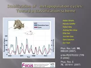
Stabilization of metapopulation cycles: Toward a classification scheme. Nadav Shnerb Marcelo Schiffer Refael Abta Avishag Ben-Ishay Efrat Seri Yosi Ben-Zion Sorin Solomon Gur Yaari. Phys. Rev. Lett. 98 , 098104 (2007). q-bio.PE/0701032 (TPB in press)

E N D
Stabilization of metapopulation cycles: Toward a classification scheme Nadav Shnerb Marcelo Schiffer Refael Abta Avishag Ben-Ishay Efrat Seri Yosi Ben-Zion Sorin Solomon Gur Yaari Phys. Rev. Lett. 98, 098104 (2007). q-bio.PE/0701032 (TPB in press) Phys. Rev. E 75, 051914 (2007)
From Herodotus of Halicarnassus to Lotka and Volterra Why the wolves do not consume all the sheep? When a wolve consumes a sheep, it becomes happier, healthier, stronger, and is more likely to breed and to produce more little wolves. The prey predator system, thus, is inherently unstable. Fifth century BCE That’s where the theory stands for about 2500y
Possible solutions to Herodotus puzzle: • It may happen that the underlying dynamics supports an attractive manifold, like limit cycle, fixed point or strange attractor • Otherwise, it may happen that the system is actually unstable, but migration between spatial patches is the stabilizing factor. This is the possibility considered here. Why?
The basic models for victim-exploiter system are unstable. Lotka-Volterra(1920’s) When the sheep population decreases, the wolves have no food anymore Population oscillations a=predator b=prey Phase portrait Fixed points: Density vs. time Conserved quantity, 1d trajectoriesmarginal stability !!
Instability: any noise drives a marginally stable system to extinction of (at least) one of the species: Random walk to extinction Q(t) is the chance that the system do not hit the walls until t, and is plotted against t for several noise amplitudes.
Nicholson - Bailey host-parasitoid model (30’s) This model is “more” unstable! Even without noise the oscillations grow until one of the species gets extinct. Bottom line: Both LV and NB models leads to an extinction of (at least) one of the species. Should it bother us?
(Old) Experimental demonstrations: growing oscillations and extinction Gause 1935:Two protist species in laboratory culture vials: Paramecium grazes on algae in the vials, Didinium preys on Paramecium Small systems are actually unstable, one of the species get extinct after a while. Pimintel flies-wasps Huffaker's (1958) oranges: 6-spotted mite and Typhlodromus
Stable oscillations in large systems: experimental (new) Holyoak & Lawler (1996) microcosms typically consist of arrays of interconnected 30-mL bottles, isolated 30-mL bottles, or large undivided bottles of the same total habitat size (not shown). The predators and prey both move freely through the interconnecting tubes. Predaor Prey
E Coli (prey) phage (predator) Kerr et. al., Nature 442 (2006)
Bacteria playing rock-paper-scissors: 3 strains of E-Coli R,S and C -Kerr et al, Nature 418 171 (2002)
So why there are stable oscillations in large systems ? … Lynx-Hare (Canada) Prickly pear cactus – cactoblastis cactorum (eastern Australia) Moose-Wolves (Isle Royal) Experiments + theory suggest that it has to do with the fact that the population is spatially structured, with patches connected by migration. But how ??
The writing was on the wall…Nicholson 1933: Predator-prey system persist, even under the influence of noise, on spatial domains connected by migration (diffusion) due to desynchronizationof different patches. Noise + Migration + Desynchronization = stability
Nicholson’s proposal - two patches example: 1. If the two patches desynchronize, then migration stabilizes the oscillations: 2. Diffusion (migration) between desynchronized patches yields a flow towards the fixed point, i.e., stabilization. 3. On the other hand, the diffusion itself tend to synchronize the two patches.
Synchronization: When oscillating systems are coupled, they tend to synchronize This happens even for mechanical coupling, not to mention diffusive coupling (density independent migration) that tends to decrease gradients !!
Two coupled LV patchesMigration induced synchronization a1(t=0) = 3 a2(t=0) = 1.5 b1(0)=b2(0) =1 D=0.2 Homogenous (invariant) manifold
The challenge:find a mechanism that maintains desynchronization in the presence of migration, thus allowing migration to be a stabilizer. “A unifying explanation or approach has remained elusive ….” [Keeling, Wilson and Pacala, Science 290 1758 (2000)] • The answers: • Spatial heterogeneity • Environmental stochasticity • Jansen’s mechanism • Noise - nonlinearity induced stability.
Spatial heterogeneity- LV q = 1.4 Gray scale – later times are darker. Same initial conditions for both patches – system initiated on the invariant manifold Constant phase Between demoi Convergence to the fixed point
Environmental stochasticity q jumps randomly between 1.4 and 0.6 Same initial conditions for both patches – system initiated on the invariant manifold Phase oscillates Convergence to the fixed point
Is that enough ?Is the stability of these systems relays on one of these mechanisms? • Systems seems to admit neither spatial heterogeneity nor environmental stochasticity. • Migration rates are more or less equal for the exploiter and the victim.
Results from individual-based simulations of predator-prey model. 100% free of any environmental differences, same migration rates, still, it seems that even demographic stochasticity may stabilize the system. Wilson, de Roos, McCauley, Theor. Pop. Bio. 43, 91 1993 Bettelheim, Agam, Shnerb Physica E 9, 600 (2001) Washenberger, Mobilia & Tauber Cond-mat/0606809 Kerr et. Al. , Nature 2006 What is going on ?
Two LV patches Single patch: servival probability Q(t) for few noise amplitudes Lifetime grows with diffusion -> appearance of an attractive manifold. What is going on ???
Noise and nonlinearity: Amplitude dependent angular velocity Noise induces amplitude differences. + Angular velocity depends on amplitude = desynchronization Phys. Rev. Lett. 98, 098104 (2007).
Coupled oscillators model for ADAV Noise yields finite distribution of r, NOW this implies different angular velocities along different trajectories. Thus <2> acquires finite expectation value, so does the “restoring force” on the invariant manifold R. This model supports all the 4 stability mechanisms. May be used to classify the underlying stabilizer using a-priory knowledge of model parameters or aposteriori measurements of species abundance.
Lotka Volterra Vs. Coupled oscillators:Lifetime as a function of migration rate Lotka-Volterrawith additive noise Coupled oscillators “Demographic stochastisity”: LV with discrete agents, using event-driven algorithm. 1000 agents per site.
Correlation length: 1D system- 64 patches DP transition??
Correlation Length-2D system DP transition? Percolation transition?
Topological effects 1D 2D
9 patches- 1D 2D
16 patches- 1D 2D
25 patches- 1D 2D
Conclusions • Many experiments suggest that at least some victim-exploiter systems are unstable (extinction-prone) in the well-mixed limit, and gain their stability due to migration between patches. • Migration stabilizes such a system only if it manage to desynchronize. However, migration itself leads to synchronization and stabilize the homogenous manifold. • Mechanisms based on spatial heterogeneity, environmental stochasticity and differences in migration rates fails to explain the apparent stability of some experimental systems and individual-based simulations. • Our mechanism – amplitude dependent angular velocity – does explain these phenomena. • For the NB dynamics (unstable on a single patch) there is critical noise level above which the system becomes stable. • The coupled oscillators system serves very nicely as a toy model for population oscillations. • Jansen’s stabilization is explained by the azimuthal dependence of the angular velocity w(q). • The wolf also shall dwell with the lamb ? וגר זאב עם כבש ? Only in a desyncronized, noisy and spatially extended environment, where the angular velocity is amplitude dependent….