Download
1 / 30
440 likes | 814 Views
Data-driven Methods for Monitoring, Fault Diagnosis, Control and Optimization. John MacGregor Ali Cinar ProSensus, Inc. Illinois Institute of Technology McMaster University. Overview.

E N D
Data-driven Methods for Monitoring, Fault Diagnosis, Control and Optimization John MacGregor Ali Cinar ProSensus, Inc. Illinois Institute of Technology McMaster University
Overview • An overall theme: Making use of historical plant data • Empirical models • Optimization • Control • Monitoring and fault diagnosis • Fault tolerant control John MacGregor Ali Cinar
Models • Mechanistic • Structure from theory / Parameters from data • Advantages are well known • Problems: • Assumptions that may be poor; theory for many y’s not known • May not incorporate many of measured variables • Examples: Y’s or X’s that are images or PAT sensors • Empirical • Structure and parameters from data • Advantages are again well known: • Problems: • Structure is often imposed and unrealistic, no interpretability nor any causality
Latent Variable Models - Concepts Measured variables Latent variable space t2 t1 X T Summary statistics: T2 and SPE (c) 2004-2010, ProSensus, Inc.
Latent variable regression models Two data matrices: X and Y Symmetric in X and Y • No hypothesized relation between X and Y • Both X and Y are functions of the latent variables, T • Choice of what is X and Y depends upon objectives X T Y X = TPT + E Y = TCT + F (c) 2004-2010, ProSensus, Inc.
Why Latent Variable Models? • Low dimensional models • Define the space containing most of the information • Simultaneously model both the X and Y spaces • Model structure truly determined by the data • This makes models unique and interpretable • Provides causal models in the low dimensional LV space • Allows for active use of the model (eg. optimization) • Allows for • easy handling of missing data • Easy detection of abnormal observations (*) • Other regression methods (MLR, ANN, etc) do not share these advantages when using historical data. • Non-unique, uninterpretable, non-causal
Optimization in Latent Variable Spaces • For active use of model, must have causality • Active use optimization / control / diagnosis • Historical plant data generally do not contain causal information on individual variables • Nor will any model built from these data • But latent variable models do provide causality in the low dimensional LV space (t1, t2, …) • Y = TCT X= TPT (t’s define Y and X) • T = XW* (To change T must move combinations of x’s) • Optimization in low dimensional LV space • Then X and Y obtained from LV’s • Illustrate concept with 2 industrial examples
Optimization: Injection molding process • GE water systems (2003) • Polyurethane film manufacture very sensitive to humidity, temperature and raw material variations • Operators periodically readjusted the process largely by trial and error • Inject ~50 parts; measure ~10 quality variables; make adjustments • Injection velocity profiles, timing sequences, etc. • Iterate until within specification • Provided a good set of data for LV modeling • Nonlinear PLS model • 20 raw material properties; 26 process variables; 10 quality variables • Models for both Y and Variance (Y)
5 39 36 37 0 38 35 34 t[2] 20 21 28 - 5 29 26 27 30 23 25 24 - 1 0 - 7 - 6 - 5 - 4 - 3 - 2 - 1 0 1 2 3 4 5 6 7 Optimization: Injection molding process • Constraints: • Humidity , temp and raw material properties constrained to their currently measured values • SPE < ϵ; T2 < T299% These ensure validity of model • Applied only when multivariate control limits violated • Results: • Readjustment in one step • Improved quality • Reduced scrap • Operational since 2004
Optimization of a batch polymerization Pilot plant data (Air Products & Chemicals) End Properties (13) time variables Z X Y batches Recipe & Initial Conditions Variable Trajectories • Very high dimensional optimization problem • Easily solved in low dimensional LV space
Optimization for new product quality • Constraints or desired values are specified for the 13 y’s • Minimize batch duration • Optimization done in the three dimensional LV space Multiple solutions for Z, X -all satisfying the y specifications, but with different batch times.
Supervisory MPC of Batch Processes • Objective: Control final product quality • Product quality only measured upon completion of batch • Control problem is thus one of • Predicting final quality from all the initial and evolving data • Making optimal mid-course corrections at several decision points during the batch (QP) • Different objectives at each decision point • PLS models have been shown to be ideal for modeling batch trajectory data and predicting final quality • Build from historical batch data • Plus some DOE runs at the decision points • Closed-loop identification used for subsequent implementations
Supervisory MPC of Batch Processes • Commercial systems in food industry > 100,000 batches controlled > 99.9% up-time > 50% reduction in std dev of all final quality attributes - 20-40% increases in productivity • LV models also allow MSPC monitoring throughout the batch. • This helps make controller robust to faults • – e.g. wireless temp sensor failure – default controllers. with ABC without ABC Final quality attribute SP
Summary (first part) • Latent variable models provide powerful ways to use historical operating data • Can make use of all measured variables • Provide unique, interpretable models for analysis • Provide causality in the LV space for optimization, control • Industrial examples used to illustrate this • Provide monitoring and diagnosis capabilities (next part)
Implementation and Automation of Process Supervision • Many variations of PCA: PCA, MBPCA, DPCA, … • Many techniques: PCA, PLS, Independent Component Analysis (ICA), … • The Irish potato famine - single kind of potato (Lumper) Diversity provides robustness • Develop a SPM, FD and control system that uses many alternate techniques • How to decide which technique works better for a given situation? Add a management layer • How to improve decision-making with experience? Use distributed AI
Adaptive, Decentralized Process Supervision Develop an agent-based monitoring, fault detection, diagnosis, and control system to: • Coordinate alternative techniques for reliable and accurate fault detection, diagnosis (FDD) and control • Improve performance via: • context-dependent performance assessment and decision-making • multi-level learning • adaptation
Distributed Artificial Intelligence • Implement with Agent-Based Systems (ABS) • Decision-making is decentralized and divided into hierarchical layers • Agents: • are autonomous software entities • observe their environment • acton their environment according to predefined rules/algorithms • may adapt by changing their rules/interpretation based on their environmental conditions at run time
MADCABS: Monitoring Analysis Diagnosis and Control with Agent-Based Systems • MADCABS is built using a hierarchical layout, with physical communication layer, processsupervisionlayer and agent management layer Basic information flow: Collection of raw data from plant Preprocessing,monitoring, diagnosis,control Mapping control actions back to process Evaluation of technique and agent performance
Process Process Monitoring • Calculates the performances: Accumulated performances of fault detection agents are summed to find the total performance of the monitoring agent • Builds new statistical models: When all monitoring agents are performing badly or the process operating mode changes. • Statistical process monitoring techniques used • Principal component analysis (PCA) • Dynamic PCA (DPCA) • Multi-block PCA (MB-PCA) Monitoring Organizer
Fault detection agents PCA_SPE PCA_T2 MB-PCA_SPE MB-PCA_T2 DPCA_SPE DPCA_T2 Process Fault Detection • Gives out-of-control signals based on the consensus formed between fault detection agents • Observes performances of fault detection agents under different fault magnitudes and keeps history • Triggers diagnosis agent • Fault detection agents are the monitoring statistics for PCA, DPCA and MB-PCA • Hotelling’s T2 and SPE statistics Fault detection organizer
Fault Diagnosis Diagnosis Manager Consensus Fault Decision Fault Detection Organizer Diagnosis Training Agent Diagnosis Agent Fault Identification Agents Database Process
Fault Type 1 SPE SPE = eeT Fault Type 1 Fault Type 2 Fault Type 2 Observation Y X For an out-of-control observation: Squared Prediction Error SPE = ∑ej , j = 1, …, number of variables N Variance between classes max 1s Fault Type 1 Variance within classes Fault Type 2 1s Variable Contributions Classify new observation based on the closeness to the existing clusters Classify new observation based on the class membership y = BPLS x X5 X3 X1 Fault Diagnosis: Identification techniques • Contribution Plots • Variable contributions to monitoring statistics T2 and SPE • Fishers Discriminant Analysis (FDA) • Partial Least Squares Discriminant Analysis (PLSDA)
Fault Diagnosis (Identification) Agents PCA_SPE [X1,X4,X7] PCA_T2 [X1,X4] MB-PCA_SPE [X1,X4] MBPCA_T2 [X1,X4,X7,X8] DPCA_SPE [X1,X4,X6] DPCA_T2 [X1,X4] Fault Signature for F1 Project the new fault data on the model and determine the most likely fault class [X1,X4] Contribution Maps [X1,X4] : [F1, F1, …] Contribution Map Estimator FDA PLSDA Identification (Discrimination) Agents Process
Agent Performance Management Layer Performance Evaluation: • Record the performance of the agent and the state metrics that define the state of the system when that performance is observed. [State Metrici, i=1,…,I ] = f (performance) • Compare the current state of the system to recorded states, and estimate the performance of the agent for the current state based on its performance for similar states in history.
Performance History Space New Data Point: What would the performances of each agent be for this state? State Metric 2 Agent A Pest,A Agent B Pest,C State Metric 1 Agent C Pest,B Pestimate For each agent: • Identify performances at closest • state points. • Obtain a performance estimate for the • current state point by interpolation. d3 d1 P3 d2 P1 P2
Diagnosis Performance History • Record: • Fault signature • Fault signatures are the process variables significantly contributing to the inflation of the monitoring statistic • Fault signatures are available once the fault is detected • Performance of the agent for that fault signature • Performance is recorded only after diagnosis is confirmed • Use the history to find: • Agents that are the best performers for the current fault signature. Diagnosis agent uses the estimated performances of fault identificationagents for the potential fault to form the consensus diagnosis decision
Adaptation:Performance-Based Consensus Analysis • Agents update their built-in knowledge and methods they use • Discriminant agents update their models with current data Contribution Map Estimator Adaptive FDA Adaptive PLSDA Over time, after a diagnosis decision is confirmed for a fault type, the misclassifications are used to update the models of the adaptive instances
Fault-tolerant Control Structures Plant orsimulator System Identification Single centralized control system PID control Set of Controllers MPC Control Decentralized control: . Local coordinated MPCs . Local MPCs integrated with local FDD modules using ABS Controller Performance Assessment Monitoring and Diagnosis
Summary/Conclusions • Latent variable models provide powerful ways to use historical operating data • Data-driven methods are well-suited for distributed process supervision • Learning and adaptation in monitoring, FDD and control enable fault- tolerant control • MADCABS provides an environment for adaptive fault diagnosis and fault-tolerant control • There are alternative approaches – Vive la difference!
Acknowledgements • IIT & ANL: • Fouad Teymour • Cindy Hood • Michael North • Arsun Artel • Inanc Birol • David Mendoza • Sinem Perk • QuanMin Shao • Derya Tetiker • Eric Tatara • Cenk Undey Financial Support by National Science Foundation CTS-0325378 of the ITR program. • McMaster University & ProSensus • Many of my former grad students at McMaster • The ProSensus team