
Numerical Models
E N D
Presentation Transcript
Numerical Models An Overview and Tutorial
Types of Models • Short range models • These tend to be more suitable for more specific features such as fronts, temperatures, and convection. They are considered non-hydrostatic. • Forecasting for as little as the next 1 hour to as long as 3 ½ days. • Long range models • These are hemispheric or global models and are highly skilled at wave patterns within the jet stream. However they also have skill at synoptic features and an outperform the short range models at times! These are usually hydrostatic or isentropic. • Forecasting out to as far as 15 days • For an understanding of terms such as hydrostatic or isentropic, we encourage you to look outside this tutorial (google it!) to get an overview.
So many models! • RUC – Rapid Update Cycle • NAM – North American Mesoscale • WRF-NMM, WRF-ARW and WRF-HRW • GFS – Global Forecast Systems • ECMWF – European Center for Medium Range Weather Forecasting • NGM – Nested Grid Model (being phased out.)
So many models! • GEM – Global Environmental Multiscale (Canada) • UKMET – United Kingdom Meteorological Model • NOGAPS – Navy Operational Global Atmospheric Prediction System • Hurricane models such as the HWRF, GFDL, and WW3
Let us narrow it down • For the purposes of this tutorial we will only concentrate on the models most used here at NEXLAB. • And they are …. • RUC • WRF • GFS • And to a certain extent the ECMWF and GEM • Oh, and there is ensemble forecasting, too. But we’ll get to that later
Rapid Update Cycle (RUC) • The RUC is a very short range model with forecasts as short as 1 hour. • Many versions of the RUC run at places such as NCEP, FSL, local weather offices, and even colleges. The operational model comes out of NCEP and is run every hour. • Every three hours (0Z, 3Z, 6Z, etc.) it runs a forecast out to 12 hours. During the hours in between it forecasts only for the next 3 hours. So, at 0Z you get forecast through 12Z but at 1Z you get a forecast valid through 4Z • Generally used for the 1, 2, 3, 6, 9, and 12 hour forecast period but as mentioned before, many versions and suites of the RUC are run so this is not always the case. But this is what you see on our website here at COD. • RUC Analyses often used for “analysis” data such as the SPC meso-analysis page so understanding the RUC can be vital in modern day forecasting.
Rapid Update Cycle (RUC) • The lastest version of the RUC (as of September 2008) has a horizontal resolution of 13km and 50 layers through the depth of the atmosphere. • Much information can be found about the RUC at http://maps.fsl.noaa.gov/
Rapid Update Cycle (RUC) This is the domain of the RUC-13km model. Data is taken a grid point spaced every 13km throughout this entire region (but only this region!)
Rapid Update Cycle (RUC) This is the 12Z RUC, 3 hour forecast of surface theta-e, valid at 15Z.
North American Mesoscale (NAM) • The NAM is the operational short range model run by NCEP. • The actual model itself is called the WRF (Weather Research and Forecasting), and more technically the WRF-NMM (Nonhydrostatic Mesoscale Model). • The WRF, like the RUC, is run different ways by different places. You may see references to the WRF-ARW (Advanced Research), too. • With all that being said, the NAM is the operational run and uses the WRF-NMM model for the basis of operational forecasting. If you see NAM or WRF, it simply means you are looking at the WRF-NMM model. • Confused yet? Don’t worry because the models are always changing names. • I encourage you to look at the WRF homepage at http://www.wrf-model.org/index.php
North American Mesoscale (NAM) • The NAM/WRF is run four times a day at 00Z, 6Z, 12Z, and 18Z. • The NAM/WRF does a forecast for every 6 hours out to 84 hours from the time it is run, or 3 ½ days. • The NAM/WRF is set up as a non-hydrostatic model run at 12km of horizontal resolution and has 60 layers through the depth of the atmosphere. • Further learning about the NAM resolution can be found at http://www.meted.ucar.edu/nwp/pcu2/namhres1.htm
North American Mesoscale (NAM) This is the domain of the WRF-12km model. Data is taken a grid point spaced every 12km throughout this entire region (but only this region!)
North American Mesoscale (NAM) This is the 12Z WRF, 6 hour forecast of QPF (precipitation), valid at 18Z
Global Forecast System (GFS) • The GFS is a short, medium, and long range model with forecasts out to 384 hours. • The GFS forecasts for every 6 hours (00Z, 6Z, 12Z, and 18Z) out to 180 hours, then every 12 hours out to 384 hours. • At 180 hours the resolution is not as fine so the user will see less detail in products beyond 180 hours. • The GFS has 64 layers throughout the depth of the atmosphere with a horizontal resolution of 30km (though 180hrs).
Global Forecast System (GFS) The GFS is a global model run for the northern hemisphere (the domain is shown above) and for the southern hemisphere. This is one reason the GFS is very skilled at wave patterns and overall jet stream flow.
Global Forecast Systems (GFS) This is the 00Z GFS, 9 day forecast of 500 speeds, valid at 00Z of day 9
The Products • Speeds (jets) • Vertical Velocity and vorticity products • Temperature fields • Humidity and moisture • Thicknesses and precipitation (QPF) • Instability and shear fields
GFS (in this case) 500mb speeds Jet maxima Heights Upper lows Ridge Wind barbs Color bar (key) The Products -- Speeds L L Products like this can be found on just about every model for major layers of the upper atmosphere such as 250mb, 500mb, 700mb, and 850mb. Some models will include a few layers in between, as well.
The Products – Vorticity • Vorticity is a complicated thing to understand. For the basis of this tutorial we will only discuss the basics. You are encouraged to learn more about vorticity on your own! • Essentially, vorticity is the spin of the air. The more the air is sheared, or spun, the higher the value of vorticity. • Vorticity is generally displayed on a 500mb map due to the fact that 500mb is in the middle of the troposphere. • When looking at a vorticity map, the center of vorticity (the maximum value) is generally associated with the heart of a shortwave trough. It might be referred to as a “vortmax” • Areas downwind of this vorticity center (where vorticity is being advected positively) can be understood to be an area of upward vertical motion. Consequently, areas upwind of the shortwave trough where vorticity is decreasing can be understood to have sinking air. Again, this is a simplified understanding of vorticity but does have practical applications.
GFS (for this case) 500mb Vorticity 500mb Heights Vorticitiy Maximum (vortmax) Shortwave troughs Color Bar The Products - Vorticity X X X X X
The Products – Vertical Velocities • The Vertical Velocity product (or VV’s or UVV’s for upward vertical velocities) is simply a measure of how much the air is rising or sinking. • This is a measure of overall rising air (synoptic) so even the fastest of vertical velocities is very small. This is not a measure of strong forcing as in a thunderstorm. The measure is done in microbars/second which is close to centimeters per second. • Two main ingredients go into measuring vertical velocities – temperature advection and vorticity advection. Warm advection and positive vorticity advection are associated with lift, or rising air. Cold advection and negative vorticity advection are associated with subsidence, or sinking air.
The Products – Vertical Velocities • Like the other products, we are using the GFS model here. • Areas of rising air • Areas of strong sinking • Also, as with previous maps and slides, the heights and color bar are located on here. Products like this can be found on most models and at many layers such as 500mb, 700mb, and 850mb. The default, or standard layer, is usually at 700mb for this product.
The Products - Temperatures • There are three main types of temperature products found on most model outputs. • Basic air temperatures (T) • Wet-bulb temperatures (Tw) – used for precipitation type. • Theta-e (Θe) – a measure of total heat (basically a combination of air temperature and moisture)
GFS (in this case) Surface (2 meter) temperatures Mean sea level pressure Highs and Lows Wind barbs You can find fronts, troughs, and ridges Tropical systems, too The Products - Temperatures H L L All models have some form of temperature forecast plot. Generally you will find this for the mid and low levels (500, 700, 850, 925) and the surface. L
The Products – Temperatures (Theta-e) An understanding theta-e is more easily attainable when one has studied soundings and the concept of parcels. What one should realize, though, is that theta-e is a measure of the total heat. The higher the value of theta-e (measured in Kelvin in this picture) the higher the heat content. In this picture to the right it is easy to see that a very cool, dry, continental air mass is taking hold of the Great Lakes region. It is important to note that theta-e values are often detailed at the surface, 850mb (as in this picture), and 700. For severe weather, we look for theta-e to decrease with height. In other words, very warm/moist at the low levels and much cooler/dryer air aloft. Concepts of theta and theta-e also involve motions of air such as isentropic lift. We encourage all students to look further into these concepts on their own (or in a class!) Cool and dry air advecting southward Southeasterly winds advect warmer and more moist air
Moisture Parameters • Relative Humidity – generally done for upper air products, 250mb-850mb. • Dewpoints – generally done for the lower layers of the atmosphere (850mb, 925mb) and near the surface.
Moisture Parameters - RH • Relative Humidity plots are done all upper levels of the atmosphere. • 250 – One might look for areas of RH to see where thick cirrus is being forecast • 500 and 700 – The model world’s version of looking at a water vapor satellite. One can see dry intrusions, areas of vertical ascent and subsidence. And a careful observer can note areas of convection blowing up within a dry intrusion. • 850 and 925 – Forecasters can use this to see areas of thick stratus and warm advection as well as general areas of vertical motion (which creates or impedes cloud development.) • Streamlines, a snapshot of the wind flow, are also plotted along with the RH to help the user in the analysis.
Moisture Parameters – Dewpoint • Dewpoint temperatures (Td) are generally plotted for the lower levels of the atmosphere such as 850mb to the surface. • Surface dewpoint plots can be calculated in different ways of which the user needs to be aware. Here at COD, we do it two ways. • 2m Td – The “skin” layer of the surface. This is the model prediction of what the surface observations will record the dewpoint to be at each hour. • 0-30mb Td – An average dewpoint of the lowest 30mb. This takes into account some mixing that goes on in the lowest part of the boundary layer. • Do not be surprised to see other parameters plotted along with the dewpoints such as streamlines, wind barbs, lifted indexes, C.A.P.E, etc. Dewpoint temperatures plots are vital to severe weather forecasting hence the severe weather overlay plots and wind plots. • Dewpoints are also very important in winter forecasting, temperature forecasts, general forecasting (clouds, etc.), among other things.
Moisture Parameters – Dewpoint This is a great example of “moisture return”. At image one (at 12Z Nov 20) one can observe a surface high pressure sitting along the coast of Louisiana and Texas. This is noted by the anticyclonic (clockwise) flow of air. With time, this high pressure moves to the east, allowing the southerly flow on the back side of the high to bring moisture from the Gulf of Mexico back into the eastern half of the US.
Thicknesses and Precipitation • Most sites that provide model data, including here at NEXLAB, tend to display thickness plots with a QPF (Quantitative Precipitation Forecast) overlay. • What is thickness? • To properly understand thickness plots, students are encouraged to further look into the hypsometric equation. A basic understanding is as follows: “The thicker the warmer”. Air expands when it is heated, and the atmosphere responds accordingly. Higher thickness values mean a higher average temperature within that layer. • A standard thickness plot is done for the 1000 – 500mb layer. However there are many others and can be seen on our models’ page. • The “540” line is a first guess, rule of thumb, for rain vs. snow. 540 is short for 5400 meters. That can, often, represent the thickness associated with an average temperature from 1000-500mb that is cold enough for snow or ice. But beware – it is not very precise. • What is QPF? • Be careful to understand that precipitation forecasts are based on precipitation that has fallen and not precipitation that is falling ! • The precipitation plot is for precip that has fallen either for the previous 3 or 6 hours. Be aware of which one you are looking at! • Just because a model says it will have precip doesn’t mean it will have it. Model world does not equal reality. Models are tools, not gospel! Do not get caught up in looking at QPF and basing your forecast completely on those plots. They are good indicators but not perfect prognostications.
QPF along with color bar. 1000-500mb thicknesses The “540” line (5400 meter thickness) is solid yellow Thicknesses and Precipitation
There are 6 thicknesses plotted, as well as the 850mb, 0 degree line. Also the average RH from 850-500mb. Each thickness rule of thumb rain vs. snow involves a different slice of the troposphere. Again, line is based on statistics that say “given this thickness, for this particular layer, the average temperature generally produces wintry precipitation.”. This is NOT the same as doing an analysis and not absolute fact. This is only one of many tools for rain vs snow. Using thicknesses to forecast
Instability and Shear Products • Many of these products involve a more in depth understanding of meteorology. • However, limited knowledge of these products can allow a user to at least get a feel for the severe weather conditions possible. • One is encouraged to further study severe weather paramaters such as shear, instability, sounding analysis, hodographs, and other severe weather analysis tools and concepts.
Instability and Shear Products • Instability products – how fast can air rise? • Convective Available Potential Energy (CAPE) – Measure in Joules of energy per Kilogram of air. The higher the number, the more unstable. Usually ranges from 25 (very low) to 5 or 6 thousand (very high). • (SBCAPE) Surface Based – air lifted upward from the ground • (MLCAPE) Mixed Layer – accounts for mixing within the boundary layer • (MUCAPE) Most Unstable (parcel) – lifts many parcels from within the boundary layer then gives the value for the most unstable lifted air. • Lifted Index (LI) – the difference in the temperature within the cumulus, or thunderstorm, vs. the temperature outside the cloud. The more negative the value, the more unstable. • Lapse Rates or Delta-T’s – shows how fast the atmosphere is cooling with height. The higher the number, the faster the atmosphere is cooling off with an increase in altitude. • (CINH) Convective Inhibition – how much will the air be suppressed? Values that are higher point to air that will be prevent air from rising due to warm air in the mid levels of the atmosphere. Also referred to as a cap or a lid on the atmosphere.
Instability and Shear Products • Shear products – how much can the air spin? • Helicity – measures shear. The higher the number, the higher the shear. • 0-6 km – an idea of “total shear” within a storm • 0-3 km – concentrates on the lower part of the atmosphere • 0-1 km – can help forecast the possibility for tornadoes One should never take these products as gospel. Shear and instability are very difficult to forecast and models are not very skilled or precise when it comes to the placement or exact numbers of instability or highly sheared areas. One should do a very good analysis before ever looking at a model! Other model packages such as BUFKIT (which we have here at the lab!) and RAOB do a wonderful job of showing a point by point vertical analysis of the atmosphere, and show CAPE and shear far better than just simple plots.
A Convective Forecast • There are three basic ingredients for convection (showers and thunderstorms). • Lift – fronts, mountains, sea breezes, shortwave troughs, etc. • Instability – high CAPE values, large negative values of LI’s, strong lapse rates, etc. • Moisture – High values of dewpoints or mixing ratio in the low levels (the boundary layer).
A Convective Forecast First, lets us understand this is the GFS and it is a 5 day forecast so there are reasons to doubt this. For the sake of this tutorial, let us just assume this is going to be correct or what we call “perfect prog” (perfect prognostication). The above is a forecast for SBCAPE valid at 18Z and 00Z. This is a fairly low instability forecast, but there is enough instability for thunderstorms and severe with CAPE’s above 1000 forecast. What do I notice here? I see a bull's-eye of CAPE in the Texas Panhandle at 18Z, then in southwest KS at 00Z. Clearly, the area of instability is in a north-south line in the western high plains of the US. This should make a forecaster aware that thunderstorms are certainly possible in that region.
A Convective Forecast This is the MLCAPE and Delta-T’s for 700mb to 500mb (one takes the temperature at a point at 700mb then subtracts the 500mb temperature from that same point to get the Delta-T, or change in Temperature. In this case, there isn’t much difference from the SBCAPE and MLCAPE. Sometimes there is. However, at 18Z you can clearly tell that the extent of CAPE above 500 J/kg is far smaller than in the SBCAPE plot. By 00Z, the MLCAPE and SBCAPE are far more similar. Why would this be? Advanced students should really being to think about why/how this could occur.
A Convective Forecast Another way to look at instability is by using the LI forecasting. This plot also can easily show you fronts based on where the LI gradient is located. Notice how packed the lines are of positive LI’s (stable air) in Nebraska, for instance. Again, this plot can confirm where the instability is. You can see the bulls-eyes and area of most unstable air. One can also note the bountiful southerly flow brining warm and moisture air into the Plains.
A Convective Forecast The question now is … “Why is the CAPE so concentrated along the western high plains? What is going on there? At this point one should have done an upper air analysis. For the sake of this tutorial we will simply show you the overall pattern at 500mb. An analysis of this shows a very large, somewhat closed, upper low centered in Montana, and lifting to the northeast. A strong jet max extends from the desert southwest into the northern plains. One should being to get a picture of what is going on. Notice the southern part of that jet is co-located with the area of CAPE you have seen in previous slides. Now you know you have an area of maximum winds aloft over an area of instability.
A Convective Forecast Now that we see what is going on in aloft we should take a look at the surface. Based on the temperatures alone, we can see some sort of frontal moving through Nebraska, Colorado, and New Mexico. An area of low pressure (a fairly weak one with pressures above 1005mb) exists in southwest KS/southeast CO. A fairly elongated area of low pressure extends from that low down into New Mexico and extreme southwestern Texas (a surface trough). Temperatures are maximized at 18Z along the front back into the Low and in southwestern Texas. This front, low, and trough are serving as an area of convergence where air is forced upward. In other words, the area where CAPE existed, and there was a jet max, also has lift. Do you notice the surface winds in the Texas Panhanldle? At 18Z they are mostly southerly but at 00Z they back (shift in a counter-clockwise direction) and our now out of the southeast? This increases the shear as winds aloft, as you saw in the previous slide, are from the southwest! Those winds are turning with height. At this point, we now we have lift and instability. Now we need to look for moisture!
A Convective Forecast Very strong southerly to easterly flow from the Gulf of Mexico and southern US is very evident on the streamlines plotted on this image. On top of that, dewpoints above 50F exist in a large area (anything in the brighter green is 50+ Fahrenheit.) Dewpoints exceeding 60F are actually quite abundant along the area of convergence along the fronts and trough. It appears a feature known as a dryline is located from southwest Kansas into southeastern New Mexico. Students are encouraged to look further into what this feature is. Regardless, it is easy to tell where winds are “piling up” or converging, and that is what is important. Those areas are located where the strongest instability exists, as well as under that 500mb jet stream maximum.
A Convective Forecast Cinh is simply the measure of stable air, or negative-CAPE, that exists which will impede the progress of upward moving air. You will notice that at 18Z the cap (areas where cinh exists) breaks in the Texas pahandle into western Kansas. You will also notice this is where, as noticed in previous slides, convergence at the low levels exists, there is plenty of moisture, shear, and instability. Is it possible that we could get convection? Could it be severe? It appears that, while the instability is weak there is at least the possibility of convection and could even be severe in nature. The cap gets stronger at 00Z but still shows some weakness with low values. Advanced students should be thinking about why this might be going on. So now we must find out how the model is handling all this information!
A Convective Forecast We have seen in the previous slides all the ingredients for thunderstorms that exist in the western high plains. Now we check to see if the model is indeed forecasting thunderstorms to develop. Can you see what the model is doing here? Precipitation is already ongoing in Nebraska at 18Z (remember that precip is accumulated from 12Z to 18Z). Remember that front moving through Nebraska? Meanwhile, from 18Z to 00Z precip moves down the trough into Texas and New Mexico. Knowing what you know, you can infer that this precipitation is likely in the form of showers and thunderstorms – convection.
A Convective Forecast • Convection that may be severe - S.L.I.M. • Shear – a change of wind speeds and/or direction over some distance. This is best done by some sounding (model or real data) analyses. But forecast helicities, or just an analysis of the jets and low level wind flow can be sufficient as an overview of the potential shear. • Lift – an ability to force the air upward. Fronts, sea breezes, mountains, etc. Generally speaking with severe, lift will be associated with fronts, drylines, surface troughs, and shortwave troughs. • Instability – conditions in place to allow air to rise on its own (air lifted must be warmer than the surrounding preexisting air in place). Don’t forget to look at CINH, too, which is an area of stability supressing convection. • Moisture – sufficient moisture in place in the low levels of the atmosphere for storms.