Download
1 / 20
200 likes | 225 Views
Explore the impact of numerical mixing in COSIMA Models through diathermal heat transport analysis. This study compares various model resolutions, mixing types, and surface forcing impacts on ocean heat transport. Findings reveal variations in numerical mixing based on model configurations.

E N D
Numerical Mixing in the COSIMA Models Ryan Holmes Jan Zika, Matthew England, Steve Griffies, Kial Stewart, Andy Hogg and others
Diathermal Heat Transport in MOM5 • Wm-2 MOM5 Eulerian heat budget diagnostics (each x,y,z,t): Integrate the heat budget over temperature layers Walin 1982 • Watts
Example: MOM025-SIS 1.6PW Surface forcing Increases temperature contrasts Downgradient heat transfer from Mixing
Example: MOM025-SIS • Numerical mixing is quantified by the heat flux that it drives between different temperature classes • Provides an estimate resolved in temperature and time • Does not require targeted simulations, or sorting • Can be extended to a horizontally-resolved (x,y,T,t) estimate of numerical mixing using lateral volume transports • What follows: Comparisons across COSIMA model suite • - 1º, ¼º and 1/10º, • - GFDL50/KDS50/75/135 • - GM/Redi on/off • - background vertical diffusivity • Seasonality:
Horizontal Resolution • Surface Forcing Note not clean comparison: • MOM025/MOM01 – CORE-NYF • ACCESS-OM2 – JRA55 RYF8585 • MOM01 = KDS75. Others = GFDL50 • Tendency • Redi Mixing • 1/4º models have largest numerical mixing • Numerical mixing reduced in MOM01 • Significantly reduced in 1-degree model • Vertical Mixing • Numerical Mixing
Vertical Resolution • Surface Forcing • ACCESS-OM2 1-degree RYF9091 • Tendency • Both vertical and numerical reduce with vertical resolution. • Changes focused at warmer temperatures • Changes reflected in reduced total transport • Redi Mixing • Vertical Mixing • Numerical Mixing
Surface Forcing Neutral Physics • ACCESS-OM2 1/4-degree RYF8485 • Tendency • Numerical Mixing reduces at cooler temperatures when Redi turned on • However, it is not reduced to zero • Turning GM on further reduces the explicit Redi mixing and numerical mixing • Redi mixing not insignificant at high temperatures, however GM effect is. • Redi Mixing • Vertical Mixing • Numerical Mixing
Background Diffusion • Surface Forcing • MOM025-SIS • Tendency • Vertical Mixing • Numerical mixing reduces with increased background diffusion • Changes focused at warm temperatures • Compensation is not complete -> Surface ocean structure impacted • In particular, tropical SSTs cool with more background mixing, driving a stronger air-sea heat flux • Numerical Mixing
Spatial Structure • Increasing Background Diffusion • No Background Diffusivity • Background Diffusivity 10-5 / 10-6 Equator • Reduced numerical mixing traced to tropics, in particular the Eastern Pacific • Large numerical heat fluxes in eddying WBC regions • Background Diffusivity 10-5 (1 year only)
Background Diffusion – Equatorial Temperature Biases • 10-5 / 10-6 Equator • 10-5 everywhere • MOM01 No Backgrounnd • No Background Diffusivity • In MOM025, 10-6 m2s-1 equatorial background diffusivity works best • In MOM01, reduced numerical mixing without added diffusion results in large biases
Summary • Diathermal framework -> nice way to quantify numerical mixing in realistic runs • MOM5 is numerically diffusive (can exceed explicit mixing) • Numerical mixing sensitive to: • Horizontal resolution • Vertical resolution (warm temperatures, tropics) • Neutral physics (cold temperatures) • Background diffusion (warm temperatures, tropics, links to TC biases) • Some questions to consider: • What are the implications of mixing numerically vs. physically? • As resolution increases, numerical mixing decreases. When do we turn on explicit mixing? • How do we balance these choices across latitude?
Spatial Structure Method • Construct budget for volume of fluid warmer than a given T within each fluid column. • 1) Lateral volume fluxes, 2) diathermal water-mass transformations (diagnosed online), and 3) tendency (diagnosed from T-snapshots). • Issues: • WMTs at T-centres while lateral fluxes at T-edges. • Tendency and lateral fluxes are noisy (requires multiple years).
Extras: Observational Diathermal Surface Forcing Calculation performed by Sjoerd Groeskamp using WOA13 climatological SSTs, CORE surface heat fluxes (which have a global ~4Wm-2 imbalance) and a solar penetration scheme due to Marel and Antoine (1994)