Download
1 / 103
1.03k likes | 1.04k Views
Wireless Networks. Ivan Marsic Rutgers University. ISO OSI Protocol Stack. Protocol at layer i doesn’t know about protocols at i 1 and i 1. Application. 4: Transport. Reliable (TCP) Unreliable (UDP). 3: Network. End-to-end (IP) Routing Address resolution. 2: Link.

E N D
Wireless Networks Ivan Marsic Rutgers University
ISO OSI Protocol Stack • Protocol at layer i doesn’t know about protocols at i1 and i1 Application 4: Transport • Reliable (TCP) • Unreliable (UDP) 3: Network • End-to-end (IP) • Routing • Address resolution 2: Link • IEEE 802.11 WiFi • IEEE 802.3 Ethernet • PPP (modems, T1) MAC 1: Physical • Radio spectrum • Infrared • Fiber • Copper
Infrastructure vs. Ad Hoc (1) (a) (b)
Infrastructure vs. Ad Hoc (2) (c) (d)
Infrared Gamma rays Visible UV X rays Freq. 1 KHz 1 MHz 1 GHz 1 THz 1 PHz 1 EHz (AM radio) MF (SW radio) HF (FM radio - TV) VHF (TV – Cell.) UHF LF SHF Freq. 30 KHz 300 KHz 3 MHz 30 MHz 300 MHz 3 GHz 30 GHz ISM UNII Freq. 902 MHz 928 MHz 2.4 GHz 2.4835 GHz 5.725 GHz 5.785 GHz Cordless phones Baby monitors (old) Wireless LANs IEEE 802.11b, g Bluetooth Microwave ovens IEEE 802.11a HiperLAN II EM Spectrum Allocation
Information Source Transmitter Receiver Destination Communication Channel Noise Source Source Data: 0 1 0 0 1 1 0 0 1 0 Input Signal: S Source Data: 0 1 0 0 1 1 0 0 1 0 Noise: N S+N Output Signal: Data Received: 1 1 0 0 1 1 1 0 1 0 Decision threshold Sampling Times: Bits in error Communication Process
Link, channel, repeater, or node Power in Power out Decibel definition
Three dots running at the same speed around the circle in different lanes: Resultant Displacement Time 60 90 30 180 0 60 120 240 300 360 30 90 150 210 270 330 Angular phase of fundamental wave Fourier Series Approximation
Phase space: / 2 Period (T) Frequency = 2 / T A Amplitude [rad / s] A 0 2 Time (t) Phase () A sin ( t ) 3 / 2 Phase Space
Communication Channel Modulator Demodulator Transmitter Receiver Error Control Encoder Error Control Decoder Source Encoder (Compress) Source Decoder (Decompress) Information Source Destination Wireless Transmission and Receiving System
01 010 0111 0110 0010 0011 011 001 90 135 0101 0100 0000 0001 90 45 180 180 10 00 100 000 0 225 270 1001 1000 1100 1101 315 270 101 111 1011 1010 1110 1111 (a) (b) (c) 11 110 00 01 135 45 225 315 10 11 Modulation—PSK
3 bits 110 3 bits 100 3 bits 010 Amplitude Time Example 2.1
Source Data: 0 1 0 0 1 1 0 0 1 0 Input Signal: Noise: Output Signal: Discrete vs. Continuous Channel (a) (b) (c)
Example 3-bit message: 1 0 1 s(t) 5 V t T A three-bit signal waveform p1(t) (1,1,1) (1,1,1) (1,1,1) (1,1,1) p2(t) s1(t) (0,0,0) (1,1,1) p3(t) s2(t) (1,1,1) (1,1,1) 0 T 2T 3T s3(t) Signals as Vectors (a) (b) (d) Orthogonal function set (Basis vectors) (c)
Geometric Representation (a) (b) (c)
N ST SR Signal Space (a) (b)
SR = ST + N O' Noise sphere, radius , centered on ST N h ST O Signal sphere, radius Locus of Error-Causing Signals (a) (b)
Error message 1,1 1,1 Valid message Error message 1,1 1,1 Valid message Error Detection and Correction (a) (b)
Wave Interactions (a) (b)
Interference & Doppler Effect (a) (b)
Plane-Earth Model (a) (b)
Delay Spread (a) (b)
Multipath Fading (2) Delay spread (2 components) Flat Fading Direct path (1 component) Doppler spread (2 components) Fast Fading Delay spread (2 components) Frequency Selective Fading
Medium Access Control (MAC) • Controls who gets to transmit when • Avoids “collisions” of packet transmissions
Collisions Receiver electronics detects collision Receiver broadcasts info about collision (jam) = total time to detect collision = RTT of the most distant station
Channel State Assumption: There is always at least one station in need of transmission Objective: Maximize the fraction of time for the “Successful transmission” state ( or: minimize the duration of “Idle” and “Collision” )
MUX Receiver Ordering of packets on higher capacity link Ordering of packets on shared medium Multiaccess vs. Multiplexing
Deterministic Schemes Static multiaccess schemes: TDMA and FDMA
txmit txmit Transmitter t t Receiver < 1 » 1 Parameter • Ratio of propagation delay vs. packet transmission time Propagation constant :
Current packet Collides with the head of the current packet Collides with the tail of the current packet tstart Vulnerable period Time tstart txmit tstart txmit Vulnerable Period • Packet will not suffer collision if no other packets are sent within one packet time of its start
Packet Arrivals 1 2 3 4 5 6 7 Time ALOHA Departures 1 2 3 4 5 6 7 Packet Arrivals 1 2 3 4 5 6 7 Time Slotted ALOHA Departures 1 2 3 4 5 ALOHA Protocols
Arrivals at Station 1 Time Time Departures Slot 1 Slot 2 Slot 3 Slot 4 Packet Time 1 Receiver k Arrivals at Station k Time Time Departures Slot 1 Slot 2 Slot 3 Slot 4 (a) – Slotted ALOHA (b) – Pure ALOHA Transmission Success Rate
Time Slots i 1 i i 1 i 2 Analysis of Slotted ALOHA (1) ASSUMPTIONS FOR ANALYSIS: • All packets require 1 slot for x-mit • Poisson arrivals, arrival rate • Collision or perfect reception (no errors) • Immediate feedback (0, 1, e) • Retransmission of collisions (backlogged stations) • No buffering or infinite set of stations(m = )
Backlogged Stations • “Fresh” stations transmit new packets • “Backlogged” stations re-transmit collided packets
ALOHA System Model (1) • In equilibrium state, system input equals system output = S = GeG
Analysis of Slotted ALOHA (2) • 0 < < 1, since at most 1 packet / slot • Equilibrium: departure rate = arrival rate • Backlogged stations transmit randomly • Retransmissions + new transmissions:Poisson process with parameter G > • The probability of successful x-mit: S=GP0,where P0=prob. packet avoids collision • No collision => no other packets in the same slot:
Efficiency of ALOHA’s S-ALOHA: In equilibrium, arrival rate = departure rate: = GeG Max departure rate (throughput) = 1/e 0.368 @ G = 1
i Unslotted (Pure) ALOHA • Assume: all packets same size, but no fixed slots • The packet suffers no collision if no other packet is sent within 2 packets long: S=GP0=Ge2G • Max throughput 1/2e 0.184 @ G = 0.5 • Less efficient than S-ALOHA, but simpler, no global time synchronization