Linear Programming
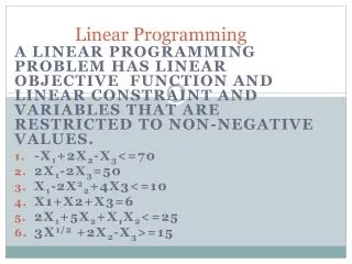
Linear Programming. Using the software that comes with the book. Let’s start with a product mix problem: Max profit 40F + 30S, subject to the constraints .4F + .5S ≤ 20 .2S ≤ 5 .6F + .3S ≤ 21 and we have the non-negativity constraints that F and S ≥ 0

Linear Programming
E N D
Presentation Transcript
Linear Programming Using the software that comes with the book.
Let’s start with a product mix problem: Max profit 40F + 30S, subject to the constraints .4F + .5S ≤ 20 .2S ≤ 5 .6F + .3S ≤ 21 and we have the non-negativity constraints that F and S ≥ 0 Here F is the product fuel additive and S is the product solvent base. Here there are three constraints to how much can be made of each of F and S. So, here we have 2 decision variables and three constraints.
The software that comes with the text can be used to solve linear programming problems. At the start you open the software and click on the Linear Programming option. You then say how many variables there are, the number of constraints (not including the non-negativity constraints), and say you are looking for a maximum value. Then you hit ok. You will then be at the input screen for the problem. Note on the objective function you have X1 and X2 generically. You can change these to F and S for our problem. Then you input the coefficients on the objective function and for the constraints. In our problem we have less than or equal to constraints, but you only have to type in the less than part. Then type in the constraints right hand side values – for example we had 20 units of material 1. You can save your work at this time. Then go to solution – solve. The output is on the next slide.
1600 is the highest profit, given the constraints F = 25 and S = 20 are the best values of F and S and make profit 1600. Section A Section B
Let’s see what the section I labeled section A means. On the computer printout this section is labeled Objective Coefficient Ranges. What we are going to do is a form of sensitivity analysis. On the F variable in our objective function we had value 40. The lower limit 24 and the upper limit 60 have the interpretation that the value of the coefficient could be anywhere from 24 to 60 and the optimal values of F and S having values 25 and 20, respectively, would not change. The profit value could change, but not these amounts. (This is assuming only the one coefficient changes.) The profit line has a slope in the graph. Changing the objective function coefficient for F changes the slope. But, as long as the change is in this range the slope does not change enough to make the optimal values of F and S change. Similarly the change of the S coefficient could go between 20 and 50 and the optimal F and S values would not change.
Simultaneous changes in the objective function coefficients If two or more (in our example we only have two) objective function coefficients change, then we may use the 100 percent rule to see if the optimal values of the decision variables change. In our example F is currently at 40 and could go up to 60 – it could go up 20 F could go down to as low as 24 - it could go down 16 and the solution would not change. Similarly S could go down 10 or up 20 from its current position of 30. Say the coefficient of F might change to 48. This is above the current spot of 40. In fact it is 8 above 40 and the allowable limit above 40 is 20 so 8 is (8/20)100 = 40% above.
Also say the coefficient of S might become 27. This is 3 below the current value of 30 and is in the allowable limit of going down 10 so 3 is (3/10)100 = 30% of the allowable decrease. The two percentage changes added together (one is an increase and one is a decrease but we just add the absolute value of the percentages) make 70% The rule – if the sum of the allowable changes is less than 100% the optimal values of the decision variables will not change. Corollary to the rule – if the sum of the changes is above 100% the optimal solution still may not change. Note: the software with the book permits editing the problem. For kicks, go to the problem and change the coefficient of F to 18 and resolve. Do you get the same solution?
Change in constraints In our example we had 3 constraints and the limiting values, or what are called the right hand sides of the constraints, were 20, 5 and 21, respectively Let’s think about one of these changing at a given time. If a value changes here, the feasible region of the solution will change. Essentially the constraint that we have a change in the right hand side for will move in a parallel fashion. This will change the size of the feasible region. Note on the printout the first constraint has slack value of zero. This means all 20 units are used. The dual price of 33.33 means for each unit change in the value of 20 changes the profit (whatever we are maximizing, in general) by 33.33. If the constraint would go up by 1 profit would go up 33.33 and if the constraint would go down by 1 profit would go down by 33.33.
The point I am making on the previous slide only holds true when the constraint changes within the limits listed on the bottom of the output. In this case the limits are from 14 to 21.5. Note the second constraint has a slack of 1. This means the constraint limit of 5 has not all been used. Consequently, having more will not change profit because what is on hand is not being totally used. The 100 percent rule and its corollary work in this area as well. Let’s do a min problem! Min 2A + 3B, subject to the constraints 1A ≥ 125, 1A + 1B ≥ 350, 2A + 1B ≤ 600, and the non-negativity constraints. The output for the problem is on the next slide.
This is a minimzation problem. Here a positive dual price means if we had a unit more of the constraining value cost would go down, by 1 in this case. A negative dual price means the cost would go up per unit increase in the constraining value.
More than two decision variables Let’s look at an example Max 40F + 30S + 50C, subject to the constraints .4F + .5S +.6C ≤ 20 .2S + .1C ≤ 5 .6F + .3S + .3C ≤ 21 and the non-negativity constraints. Let’s see the output on the next slide.
Note the optimal value of S is zero here. The reduced cost amount is 12.5. This means that the coefficient on S in the objective function would have to go up by at least 12.5 before S has a value above zero in an optimal solution. Note: If this happens the maximum value will likely change. By the way, this can happen with only two decision variables.
Constraints in Percentage terms Say in our three decision variable problem that we have another constraint of the following nature: The amount of S made must be at least 25% of the amount of F made. Thus S ≥ .25F and in the context of the computer program the constraint should be written - .25F + S ≥ 0. I will add this constraint to the problem and show the output on the next slide.
Remember we had as a constraint -.25F + S ≥ 0. The minus 12.121 means that if S was made to be 1 unit above .25F, or really constraint -.25F + S ≥ 1, Then the maximum value of the objective would fall by 12.121. Similarly, if S was made to be 1 unit below .25F the maximum value would rise by 12.121. Remember all our statements are in context of being within lower and upper limits.

